PHIL 109 · Introduction to Formal Reasoning and Decision Making
10 Games
This chapter turns to games, decisions in which the outcome depends on the choices of other agents, and shows how to represent them as matrices and trees under the standard assumptions of game theory. It then introduces the main tools for solving them (iterated deletion of dominated strategies, Nash equilibrium and saddle points, and backwards induction) and examines the Prisoner’s Dilemma, its connection to Newcomb’s problem, and the centipede game.
10.1 Games as interactive decisions
So far, every decision we have considered has been made against a partition of states of nature: possibilities that, for the most part, obtain or fail to obtain independently of what the agent decides to do. Whether it rains has nothing to do with whether you go to the park or to the movies; whether a given company’s stock rises has nothing to do with which stocks you bought. This independence is what let us treat the probability of a state as fixed, no matter which option we were evaluating.
We did, however, come across an exception to this pattern. Recall the lazy student: whether he studies is not independent of whether he passes, since studying raises the probability of passing. Even there, though, something important was still missing that will now become central. The state—passing or not passing the class—was not itself anyone’s choice. It was just a fact about the world that happened to be sensitive, probabilistically, to what the student did. Nobody was choosing to fail the lazy student in order to satisfy their own preferences.
Games are what you get when you take that last step: when the “state” that determines how well your choice turns out is not a brute fact about the world, nor even a fact that is merely sensitive to your choice, but is itself the deliberate choice of another agent—an agent who, exactly like you, has preferences over the possible outcomes and is choosing with an eye to satisfying them. This is what makes games distinctive, and it is why we call them interactive decisions.
Definition 10.1. Game: A game is a decision problem in which the relevant partition is made up not of states of nature, but of the possible choices of one or more other agents, each of whom has preferences over the possible outcomes and chooses with an eye to satisfying them. We will also call a game an interactive decision.
Because a game has more than one decision-maker, we need more than one utility function: one per player. For now we restrict ourselves to games with exactly two players, whom we will call Row and Column—names that will make sense once we get to the matrix representation below. For the sake of ease of exposition, we will also assume that Row is a man and Column is a woman. Row’s utility function will be written , and Column’s . Both take as arguments a pair consisting of a choice by Row and a choice by Column: is how good the outcome is for Row, by Row’s own lights, when Row picks and Column picks ; and is how good that very same outcome is for Column, by Column’s lights.
The rest of this chapter will make heavy use of two ways of depicting a game: as a matrix, and as a tree. We introduce the general schema for each before putting both to work on a simple example.
10.1.1 Matrices
The most compact way of representing a two-player game is as a matrix. Row’s available choices, , label the rows; Column’s available choices, , label the columns. Each cell of the resulting payoff matrix corresponds to one possible outcome—one for each combination of a choice by Row and a choice by Column—and so it must contain two utilities rather than one. We will adopt the following convention throughout: Column’s utility goes in the upper-right corner of the cell, and Row’s utility goes in the lower-left corner. Table 10.1 displays the general schema.
Reading across a row tells you how well Row does against each of Column’s possible choices; reading down a column tells you how well Column does against each of Row’s possible choices. This is exactly the kind of information a single agent’s decision matrix gave us in earlier chapters; the only novelty is that we now have two such matrices at once, layered into a single grid of cells.
10.1.2 Trees
Matrices are compact, but they hide the order, if any, in which the players choose, and they picture both players as choosing simultaneously and independently of one another. A second way of representing a game, its extensive form or game tree, makes the order of choice explicit. In a game tree, each point at which a player must choose is drawn as a circle, labeled with whichever player chooses there— for Row, for Column; the branches leading out of a node, each labeled with the choice it represents, are the options available to that player; and the tips of the branches are the possible outcomes, each labeled with a pair of utilities , in that order. Figure 10.1 gives the schema for a two-player game in which Row chooses first, among , and Column then chooses, among , already knowing what Row chose.
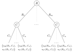
Notice the qualification at the end of the last paragraph: in Figure 10.1, Column chooses after Row, branching out separately beneath each of Row’s choices, and so is implicitly pictured as knowing what Row chose before choosing herself. That is a fine way of depicting a genuinely sequential game. But many of the games that interest us—including the one we turn to next—are not sequential: both players choose at the same time, each in ignorance of what the other is doing. A tree can still represent such a game, but only if we add a device for marking that several nodes are, from the point of view of the player choosing at them, indistinguishable. We do this by joining those nodes with a dotted line; the resulting cluster is called an information set. A player choosing at an information set must choose the same way at every node in it, since she cannot tell which one she is actually at. We will have more to say about information sets later on; for now, the dotted line is just a reminder that a choice is being made in ignorance of another player’s choice.
10.1.3 Example: Rock-Paper-Scissors
Let us put both representations to work on a simple, familiar game. In Rock-Paper-Scissors, Row and Column simultaneously choose one of Rock, Paper, or Scissors. Rock beats Scissors, Scissors beats Paper, and Paper beats Rock; if both players make the same choice, the game is a tie. The winner receives a utility of , the loser a utility of , and both players receive in the event of a tie.
Table 10.2 gives the matrix representation of the game.
| Rock | Paper | Scissors | |
|---|---|---|---|
| Rock | |||
| Paper | |||
| Scissors |
Figure 10.2 gives the tree representation of the very same game. Since Rock-Paper-Scissors is a simultaneous game, Column’s three choice nodes—one beneath each of Row’s choices—are joined by a dotted line, marking them as a single information set: Column must choose among Rock, Paper, and Scissors without having seen what Row chose.
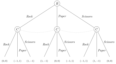
The two representations agree, as they must, on every outcome: if Row plays Scissors and Column plays Paper, both the matrix and the tree tell us that Row gets a payoff of and Column a payoff of . Which representation is more convenient depends on the game and on what we want to do with it; we will use both freely throughout this chapter.
10.1.4 From trees to matrices, and back
Before we show how to translate one representation into the other, it helps to make explicit something that has so far been true without needing a name. In both Figure 10.1 and Figure 10.2, each player moves exactly once, so a row or a column of a matrix, and a first- or second-level branch of a tree, already amounts to a complete plan of action for that player. Once players may move more than once, this stops being true, and we need the more general notion of a strategy.
Definition 10.2. Strategy: A strategy for a player in a game is a complete plan of action for that player: a specification of what she would do at every point in the game—or, if several of her decision nodes belong to the same information set, at every information set of hers—at which it might be her turn to move.
In every game we have considered so far, each player has exactly one decision node (or one information set), so a strategy for Row just is one of , and a strategy for Column just is one of . The rows and columns of our matrices, and the branches of our trees, already are strategies. This is what lets the translation between the two representations be a matter of bookkeeping rather than something requiring us to introduce anything new. The bookkeeping goes as follows.
From a tree to a matrix. List Row’s strategies along the rows and Column’s strategies along the columns. For each pair of strategies—one for Row, one for Column—follow the tree from the root, letting each player move exactly as her strategy specifies; this traces a unique path down to a single leaf. Copy that leaf’s pair of utilities into the corresponding cell of the matrix. This is exactly how Table 10.2 was read off Figure 10.2: the strategy pair (Scissors, Paper), for instance, traces a path down the branch labeled Scissors and then the branch labeled Paper, landing on the leaf labeled —which is exactly the entry in the Scissors row and Paper column of Table 10.2.
From a matrix to a tree. A matrix does not, by itself, say in what order, if any, the players moved; a tree, by contrast, always shows branches emerging from a root in some order. Turning a matrix into a tree therefore requires an arbitrary choice: pick one player to draw as moving “first” (it does not matter which), draw her strategies as the branches out of the root, and then, beneath each of those branches, draw a node for the other player, with her own strategies as its branches. If, as is usually the case, the matrix represents a genuinely simultaneous choice, join all of the second mover’s nodes into a single information set with a dotted line, exactly as we did for Column in Figure 10.2: this cancels out the false impression, created by the tree’s left-to-right layout, that the second mover already knows what the first one did. The leaves are then labeled directly from the matrix: the leaf at the end of the path through and gets whichever pair of utilities sits in row , column of the matrix.
Since Table 10.2 and Figure 10.2 depict the very same game, running either procedure on one of them should return (up to the arbitrary choice of who is drawn as moving first) the other. We encourage you to check this for yourself.
10.2 The assumptions of game theory
Before going any further, it is worth making explicit several assumptions that classical game theory takes for granted. None of them is beyond dispute—each has been challenged, by philosophers and economists alike—but we will adopt all four for the remainder of this chapter, since doing so is what lets us use matrices, trees, and the solution concepts to come in their standard form.
Utilities are measured on interval scales. Recall that an ordinal utility function only records a ranking of outcomes, whereas a cardinal, or interval-scale, utility function also records facts about the magnitude of the differences between them—and that this is exactly what maximizing expected utility requires (Norm 8.4). We will assume throughout that each player’s utility function is at least interval-scale: and are each fixed only up to a positive linear transformation (Definition 8.1), so nothing follows from the bare fact that, say, while . Comparisons of magnitude are licensed only within a single player’s own scale—Row’s against one of Row’s other numbers—never across players: classical game theory does not assume any way of comparing how much Row wants something to how much Column wants something.
Players maximize expected utility. Row and Column are both assumed to be maximizing expected utility (Norm 8.4), exactly as the single agents of earlier chapters did. It is worth being careful about what this assumption does, and does not, say. It does not say that a player always wants to win, in whatever sense her opponent would recognize as winning. A mother playing chess against her young son may well prefer that he win, and so assign a higher utility to that outcome than to her own victory. Game theory has no trouble representing this: it simply means that the mother and son are not playing the game that two rival grandmasters would be playing, even though the legal moves of chess are exactly the same in both cases. A game, recall, is individuated by the players’ utilities over outcomes, not by the nominal activity they happen to be engaged in (Definition 10.1); change the utilities and, officially, you have changed the game, whatever the rules on the box say.
All of this is common knowledge. It is not enough that the rules, the payoffs, and each player’s rationality merely happen to be known by both players; game theory assumes something considerably stronger.
Definition 10.3. Common knowledge: A proposition is common knowledge among a group of agents if and only if every agent in the group knows , every agent knows that every agent knows , every agent knows that every agent knows that every agent knows , and so on, without end.
This is a much stronger condition than what is called mutual knowledge: the mere fact that each member of a group individually knows . Suppose I tell Row, in private, that Column is rational, and I separately tell Column, in private, that Row is rational. Then it is true that both know that the other is rational—the fact is mutually known. But neither of them knows that I told the other: for all Row knows, Column may think Row is irrational, and so Row cannot safely reason about what a rational Column will do on the assumption that Column is reasoning about a rational Row. Had I announced the very same fact publicly, with both of them present and aware of each other’s presence, it would have become common knowledge instead: each would know it, each would know that the other knows it, each would know that the other knows that they know it, and so on—because each can see that the other was there to hear the announcement, and can see that the other can see this too. It is this whole infinite hierarchy, not the mere fact that everyone happens to know, that licenses each player’s confidence in reasoning about what the other player, reasoning in turn about her, will do.
We limit ourselves to two-person games. For the rest of this chapter, every game we consider will have exactly two players, Row and Column, and no more. This is a substantive restriction—many interesting games have three or more players—but it keeps our matrices and trees to a manageable size, and the theory of games with more than two players is, in any case, considerably more complicated.
10.3 Strictly competitive two-player games
Look back at Table 10.2. Every one of its nine cells has the same curious feature: whatever number appears as Row’s utility, Column’s utility is exactly that number’s negative. A win for Row () is paired with a loss for Column (); a loss for Row () is paired with a win for Column (); a tie () leaves them both exactly where they started (). Rock-Paper-Scissors is the simplest possible case of a wider phenomenon: games in which the players’ preferences are in exact opposition, so that to whatever extent one of them gains from an outcome, the other loses.
Definition 10.4. Strictly competitive: A two-player game is strictly competitive if the players’ preferences are in exact opposition: for any two outcomes, or lotteries over outcomes, and , Row prefers to if and only if Column prefers to .
Since each player’s utility function is fixed only up to a positive linear transformation (our first assumption above), it makes no sense to ask whether Column’s utility is “really” the negative of Row’s. But in a strictly competitive game we are free to choose Column’s utility function so that it is: letting be Row’s utility for a given outcome, we can take Column’s utility for that same outcome to be , so that for every and . A game whose utilities are written in this way is called zero-sum. Every strictly competitive game can be written as a zero-sum game, and so we will use the two terms interchangeably from now on.
Since Column’s utility is never independent information in a strictly competitive game—once we know Row’s utility for an outcome, we know Column’s for free, as its negative—we will simplify our matrices from here on by writing only Row’s utility in each cell and leaving Column’s implicit. Table 10.3 gives Rock-Paper-Scissors in this simplified notation. Compare it with Table 10.2 to confirm that no information has been lost: Column’s utility in any cell can always be recovered just by flipping the sign of the number written there.
| Rock | Paper | Scissors | |
|---|---|---|---|
| Rock | |||
| Paper | |||
| Scissors |
10.4 Nonzero-sum games
Not all two-player games are zero-sum. Suppose, for instance, that Row and Column want to meet during this weekend, but cannot communicate. The options, which they arranged beforehand, are to go to the park or to the movies. They both prefer meeting each other to not meeting, but Row prefers meeting at the park and Column meeting at the movies:
| Park | Movies | |
|---|---|---|
| Park | ||
| Movies |
10.5 Iterated deletion of dominated strategies
What are the norms for rational game players? One uncontroversial norm is that rational players do not play strongly dominated strategies. Remember our definition of a strongly dominated strategy from Chapter 7: option strongly dominates option if and only if does better than no matter which state obtains (Definition 7.8), that is, if and only if, for every state , In a game, the role of the states is played by the other player’s strategies. From Row’s point of view, what he does not control, and what together with his own choice settles the outcome, is which strategy Column plays; and the same goes, the other way around, for Column. So Row’s strategy strongly dominates his strategy if and only if, for every strategy of Column’s, and Column’s strategy strongly dominates her strategy if and only if, for every strategy of Row’s, In a zero-sum game written, as we have agreed, with Row’s utilities only, the second condition has to be read with care. Since Column’s utility is the negative of Row’s, Column’s strategy strongly dominates if and only if, for every , That is, every number in column is lower than the corresponding number in column . Column, remember, wants the numbers in the matrix to be as low as possible.
The dominance norm (Norm 7.10) tells us that a rational player never plays a strongly dominated strategy. Consider, then, the following zero-sum game:
None of Row’s strategies is strongly dominated: does better than if Column plays (), but worse if she plays (); does better than both of the others against , but worse than both against . Column, however, has a strongly dominated strategy: every number in column is higher than the corresponding number in column (, , and ), so strongly dominates . A rational Column, therefore, will not play .
If the dominance norm were all we had to go on, that is where our analysis would stop. But recall our third assumption: the players’ rationality, and the payoffs of the game, are common knowledge (Definition 10.3). Since Row knows that Column is rational, he knows that Column will not play , and so he can reason as if had been deleted from the game. And in the smaller game that results, is strongly dominated, by ( and ). The only thing that protected was its good showing against , and is no longer a live possibility. So a rational Row who knows that Column is rational will not play .
The process does not stop there. Column knows that Row is rational and that Row knows that Column is rational, so she, too, can work out that Row will not play , and can reason as if both and had been deleted. In the game that is left, is strongly dominated by ( and ): was protected only by the that Row would get by playing , and Row will not play . So Column deletes as well.
Finally, Row can follow all of this reasoning, so he knows that Column will play ; and against , does better than (). So Row deletes . The only strategies left standing are and , and the outcome of the game is that Row receives (and Column, therefore, ).
Try it in the Games Lab Step through iterated deletion of strongly dominated strategies in this game.
Notice how each step of this reasoning requires one more layer of knowledge than the one before. The first deletion requires only that Column be rational. The second requires, in addition, that Row know that Column is rational. The third requires that Column know that Row knows that Column is rational. And the fourth requires that Row know that Column knows that Row knows that Column is rational. In bigger games, the chain can get as long as you like, which is why game theory does not stop at any particular layer and simply assumes common knowledge, which delivers all of the layers at once.
Definition 10.5. Iterated deletion of strongly dominated strategies: Delete every strategy, of either player, that is strongly dominated. Then look at the smaller game that results and delete every strategy that is strongly dominated there; and so on, until no strongly dominated strategies remain.
Iterated deletion works in exactly the same way in games that are not zero-sum. The only difference is that we can no longer write just one number per cell, so we have to be careful to read each player’s own utilities: Row’s strategies are compared using the numbers in the lower-left corners, and Column’s using the numbers in the upper-right corners. And since those upper-right numbers are now Column’s own utilities, Column wants them to be as high as possible. Consider the game in Table 10.10.
This time it is Row who has a strongly dominated strategy to begin with: is strongly dominated by (, , and ), and also by (, , and ). None of Column’s strategies is dominated yet: does better for Column than against and , but worse against (). Once Column knows that Row will not play , however, is strongly dominated by ( and ), so she deletes it. With gone, Row loses the one thing that made worth considering, its against , and is now strongly dominated by ( and ). Finally, with only left for Row, is strongly dominated by (). The game is dominance solvable: Row plays , Column plays , and they receive and respectively. Figure 10.3 summarizes the process.
Try it in the Games Lab Step through iterated deletion of strongly dominated strategies in this game.
Something happens in this game that could never happen in a zero-sum game. Look at the outcome of and : Row would get and Column would get , so both players would be better off there than at the solution of the game. Why, then, can they not get there? Because is not stable. If Column plays , Row does better by switching to ( rather than ), which would leave Column with ; and Column, who can see this coming, will not expose herself to that risk by playing . In a zero-sum game the question cannot even arise, since there whatever is better for one player is worse for the other, so no outcome can be better for both players than another. Once we leave zero-sum games behind, by contrast, perfectly rational players, with common knowledge of each other’s rationality, can end up at an outcome that both of them would gladly trade for another one. We will see a starker version of this phenomenon when we come to the Prisoner’s Dilemma.
If, at the end of this process, each player is left with a single strategy, as happens in the two cases we examined in this section, we say that the game is dominance solvable, and we take the surviving pair of strategies to be its solution. Because we only ever delete strongly dominated strategies, the order in which we carry out the deletions makes no difference: whichever strongly dominated strategy we delete first, we always end up with the same strategies at the end. The same is not true, as we will see, if we also delete weakly dominated strategies, where the order of deletion can affect the result.
Not every game is dominance solvable, however. In Rock-Paper-Scissors (Table 10.3), no strategy of either player is strongly dominated, or even weakly dominated: each of Row’s strategies is the best possible against one of Column’s strategies and the worst possible against another, and likewise for Column. So iterated deletion does not even get started, and we would need other tools to say anything about how such games should be played.
10.6 Nash equilibrium
Iterated deletion of dominated strategies is a powerful tool, but it only gets started if some player has a dominated strategy. Consider the zero-sum game in Table 10.11, written, as usual, with only Row’s utilities.
Try it in the Games Lab Star the best responses and find the Nash equilibria step by step.
No strategy here is dominated, not even weakly. Each of Row’s strategies is his best option against one of Column’s ( against , against , and against ), and each of Column’s strategies is her best option against one of Row’s ( against , against , and against ). So iterated deletion is of no help. Can the players nevertheless figure out what to do?
Since what is best for each player depends on what the other one does, it is natural for each of them to start by asking what the other will do. Suppose, for instance, that Row expects Column to play . Then his best reply is , which would get him . But Column knows that Row is rational, and she knows the payoffs, so she can work out that if Row expected her to play he would play ; and against , her best reply is not but , which holds Row down to . The expectation that Column will play undermines itself: if Row acted on it, Column, anticipating this, would not play after all. The same thing happens if Row expects Column to play : his best reply is , which would get him , but Column’s best reply to is , which holds him down to . In fact, these expectations chase each other round in a circle: leads to , which leads to , which leads to , which leads back to .
Things are different if Row expects Column to play . His best reply to is , and Column’s best reply to is itself, since is the lowest number in row . Here, and only here, the expectation confirms itself: if Row expects and therefore plays , then Column, who can anticipate this, has every reason to play , which is just what Row expected her to do. Running the same reasoning from Column’s side singles out the very same pair. Once the players are at , neither has any reason to move: Row gets , and switching would get him only or ; Column holds Row down to , and switching would let him have or .
Notice that this solution is not particularly glamorous for Row. holds out the prospect of and the prospect of , whereas the best can do is . But Row cannot count on getting or : those outcomes require Column to play into his hands, and she has no reason to do so.
The same kind of reasoning works in games that are not zero-sum. In the game of Table 10.12, again, no strategy of either player is dominated.
Try it in the Games Lab Star the best responses and find the Nash equilibria step by step.
Suppose that Column expects Row to play . Her best reply would then be , which gets her (rather than or ). But Row, anticipating this, would play against , since that gets him (rather than or ). Against , however, Column would rather play ( rather than or ); against , Row would rather play ( rather than or ); and against , Column would rather play ( rather than or ). At this point the chain of reasoning comes to rest, since Row’s best reply to is itself ( rather than or ). The pair is the only one at which each player’s strategy is a best reply to the other’s, and wherever we start the chain of reasoning, it ends there. Each player gets .
Sometimes, however, this kind of reasoning does not single out a unique pair of strategies. Go back to the Park or Movies game (Table 10.4):
| Park | Movies | |
|---|---|---|
| Park | ||
| Movies |
Try it in the Games Lab Star the best responses and find the Nash equilibria step by step.
If Row expects Column to go to the park, his best reply is to go to the park too ( rather than ); and if Column expects Row to go to the park, her best reply is to go there as well ( rather than ). So (Park, Park) confirms itself. But so does (Movies, Movies): if each expects the other at the movies, each does best by going there too (Row gets rather than , and Column rather than ). The two remaining pairs do not confirm themselves: whoever expects the other at the park does best by going to the park, and whoever expects the other at the movies does best by going to the movies, so neither player has any reason to stick to a pair in which they miss each other. The reasoning that served the players so well in the previous two games thus leaves them, in this one, with two candidate solutions, and nothing in the game itself tells them which one to aim for. Worse, Row prefers one of them and Column the other. If each heads for his or her own favorite, they end up at (Park, Movies) and miss each other; and if each gallantly defers to the other, they end up at (Movies, Park) and miss each other again.
The self-confirming pairs of strategies we have been looking for are named after the mathematician John Nash, who introduced the idea in 1950. To state the definition precisely, we first need the notion of a best response.
Definition 10.6. Best response: A strategy of Row’s is a best response to a strategy of Column’s if and only if no strategy of Row’s does better against ; that is, if and only if, for every strategy of Row’s, Likewise, is a best response to if and only if, for every strategy of Column’s,
Definition 10.7. Nash equilibrium: A pair of strategies is a Nash equilibrium if and only if is a best response to and is a best response to .
Equivalently, a pair of strategies is a Nash equilibrium just in case neither player could do better by switching to another strategy while the other player sticks to hers. is the only Nash equilibrium of Table 10.11, and the only one of Table 10.12; Park or Movies has two, (Park, Park) and (Movies, Movies). You can also check that the solutions we found by iterated deletion in Table 10.5 and Table 10.10 (both of which happen to be ) are Nash equilibria. This is no accident: whenever iterated deletion of strongly dominated strategies leaves each player with a single strategy, the resulting pair is a Nash equilibrium, and it is the game’s only one.
Things are different if we also delete weakly dominated strategies. Consider the game in Table 10.14.
Try it in the Games Lab Star the best responses and find the Nash equilibria step by step.
This game has two Nash equilibria. At , Row’s best response to is ( rather than ), and Column’s best response to is ( rather than ). At , Row’s best response to is , since it gets him and would get him no more than that, and Column’s best response to is ( rather than ). Notice, moreover, that is better for both players than . But is weakly dominated by : against , does better (), and against the two do equally well (). If we delete on that basis, Column is left choosing between and against alone, and now is strongly dominated by (). The procedure thus leaves us with , and the equilibrium that both players prefer has been deleted along the way.
What has gone wrong? Deleting because it is weakly dominated makes sense only if Row takes seriously the possibility that Column will play , since that is the only case in which does better than . But if Row is confident that Column will play , as he is entitled to be at the equilibrium , then he loses nothing by playing . Strongly dominated strategies never raise this problem. A strongly dominated strategy does worse than some alternative against everything the other player might do, so it is never a best response to anything, and so it can never be part of a Nash equilibrium. Deleting strongly dominated strategies, however many times we do it, therefore never deletes an equilibrium. This is a second reason, in addition to the fact that the order of deletion can matter, to restrict iterated deletion (Definition 10.5) to strongly dominated strategies.
Not every game has a Nash equilibrium if we consider just the strategies depicted in the matrix corresponding to the game, however. Consider Rock-Paper-Scissors once more (Table 10.3), and go through each of the nine pairs of strategies:
| Rock | Paper | Scissors | |
|---|---|---|---|
| Rock | |||
| Paper | |||
| Scissors |
In every one of them, at least one of the players would do better by switching. At (Rock, Rock), Row would rather switch to Paper ( rather than ); at (Rock, Paper), Row would rather switch to Scissors ( rather than ); at (Rock, Scissors), Column would rather switch to Paper (getting rather than ); and so on for the remaining six pairs. Whatever pair the players expect, one of them has a reason to depart from it, and the reasoning goes round in circles forever, just as it did for the strategies other than and in Table 10.11.
This is not quite the end of the story. Instead of simply choosing one of their strategies, players can also randomize: Row could, for instance, roll a die and play Rock if it lands or , Paper if it lands or , and Scissors if it lands or . A way of choosing among one’s strategies with given probabilities is called a mixed strategy; by contrast, the strategies we have been dealing with so far are called pure strategies, and what we have defined is, strictly speaking, a Nash equilibrium in pure strategies. Nash proved that every game with finitely many players and strategies has at least one Nash equilibrium once mixed strategies are allowed. In Rock-Paper-Scissors, for instance, the only equilibrium is the one in which each player plays each strategy with probability : if Column does this, every strategy of Row’s has the same expected utility, , so Row has nothing to gain by doing anything else, and the same goes for Column. We will not deal with mixed strategies in this book, however. From now on, “Nash equilibrium” will always mean Nash equilibrium in pure strategies.
10.6.1 Saddle points
In zero-sum games, there is a simple, mechanical way of finding Nash equilibria. Recall that, in a zero-sum matrix written with Row’s utilities only, Row wants the numbers to be as high as possible and Column wants them to be as low as possible. So Row’s best response to a column is whichever row has the largest number in that column, and Column’s best response to a row is whichever column has the smallest number in that row. A pair is therefore a Nash equilibrium just in case the number in its cell is at once the largest in its column and the smallest in its row.
Definition 10.8. Saddle point: In a zero-sum game written with Row’s utilities only, a cell is a saddle point if and only if its number is both the smallest number in its row and the largest number in its column.
The name comes from the shape of a horse’s saddle: the middle of the seat is the lowest point as you move from the horse’s head to its tail, but the highest point as you move from one of its sides to the other. In a zero-sum game, then, the Nash equilibria are exactly the saddle points.
To find the saddle points of a zero-sum game, write down the minimum of each row and the maximum of each column, as in Table 10.16. The minimum of a row is what Row can guarantee himself by playing it, whatever Column does; the largest of these row minima, which is called the maximin of the game, is therefore the most Row can guarantee himself. Choosing a row whose minimum is the maximin is just following the maximin norm of Norm 7.13, with Column’s strategies playing the role of the states. Similarly, the maximum of a column is the most Row can get if Column plays it; the smallest of these column maxima, which is called the minimax of the game, is therefore the least that Column can guarantee to hold Row down to. (Since Column’s utilities are the negatives of Row’s, choosing a column whose maximum is the minimax is just Column following the maximin norm from her own point of view.)
| Row minimum | ||||
|---|---|---|---|---|
| Column maximum |
Try it in the Games Lab Step through the row minima, the column maxima and the saddle points.
In Table 10.16, the maximin and the minimax are both , and the cell where the maximin row and the minimax column meet, , is a saddle point: is the smallest number in row and the largest in column . It is, of course, the equilibrium we reasoned our way to earlier. (You can check that the solution of Table 10.5, whose value is , is a saddle point as well.)
The maximin can never be larger than the minimax. Take any row and any column : the minimum of is at most the number in their shared cell, which is in turn at most the maximum of . So every row minimum is less than or equal to every column maximum, and in particular the largest row minimum is less than or equal to the smallest column maximum. When the two are equal, the game has a saddle point, at the intersection of any row that achieves the maximin with any column that achieves the minimax. When the maximin is strictly smaller than the minimax, the game has no saddle point, and so no Nash equilibrium. Rock-Paper-Scissors is a case in point: every row minimum is and every column maximum is , so the maximin, , falls short of the minimax, .
There is something striking about all this. When we first met the maximin norm, in decisions under ignorance, it could look excessively pessimistic: why assume that the worst state will obtain? In a zero-sum game, however, the “states” are chosen by an opponent whose interests are exactly opposed to yours and who can anticipate what you will do, so expecting the worst is just being realistic. And whenever a zero-sum game has a saddle point, each player’s cautious maximin choice is exactly an equilibrium choice: neither of them could do better by being less cautious.
Finally, zero-sum games never confront the players with the problem we saw in the Park or Movies case. A zero-sum game may have more than one saddle point, but all of them have the same value (namely, the maximin, which equals the minimax); and if and are both saddle points, then so are and . So each player can simply pick any of his or her equilibrium strategies, without any need to coordinate with the other.
10.6.2 Finding pure equilibria by starring best responses
The saddle-point method only works for zero-sum games. Fortunately, there is an equally mechanical method that works for every game, zero-sum or not, and that follows the definition of a Nash equilibrium very closely. To see how it works, consider the game in Table 10.17, in which each player has five strategies.
We could, of course, go through all twenty-five cells one at a time, asking of each whether either player would do better by switching. But there is a quicker way, which consists of two passes through the matrix.
In the first pass, we go through the matrix column by column, and in each column we put a star next to Row’s highest number, that is, next to the highest of the numbers in the lower-left corners. A star on Row’s number in the cell of and thus records that is a best response to : against , no other strategy of Row’s does better. In column , for instance, Row’s numbers are , , , , and , so we star the in row . If several of Row’s numbers are tied for highest in a column, we star all of them, since each of the corresponding strategies is a best response to that column. This happens in column , where Row’s in row and his in row both get a star. The result of the first pass is shown in Table 10.18.
In the second pass, we go through the matrix row by row, and in each row we put a star next to Column’s highest number, that is, next to the highest of the numbers in the upper-right corners. A star on Column’s number in the cell of and records that is a best response to . In row , for instance, Column’s numbers are , , , , and , so we star the in column . Notice the switch: Row’s stars are assigned column by column, because what we are looking for is Row’s best response to each of Column’s strategies, whereas Column’s stars are assigned row by row, because what we are looking for is Column’s best response to each of Row’s strategies. The result of the second pass is shown in Table 10.19.
Try it in the Games Lab Star the best responses and find the Nash equilibria step by step.
Now look for the cells in which both numbers are starred. In Table 10.19 there are two: and . These are the Nash equilibria of the game, and it is easy to see why a cell with two stars is guaranteed to be one. The star on Row’s number in the cell of and tells us that is a best response to , and the star on Column’s number tells us that is a best response to . But that is exactly what it takes, according to Definition 10.7, for to be a Nash equilibrium. The reasoning also runs in the other direction: if is a Nash equilibrium, then is a best response to , so Row’s number in that cell gets a star in the first pass, and is a best response to , so Column’s number gets a star in the second. So the method finds all the pure Nash equilibria of a game, and only them. In particular, if no cell ends up with two stars, the game has no Nash equilibrium in pure strategies.
The cells with just one star are instructive too. At , Row is doing as well as he can given Column’s choice, so his number is starred; but Column is not, since against she would rather switch to ( rather than ). At the situation is reversed: Column’s is the best she can get against , but Row would rather switch to ( rather than ). A cell with only one star is one in which one of the players has a reason to switch, and that is enough to keep it from being an equilibrium. Notice, finally, that high numbers do not make an equilibrium: gives both players , exactly as much as the equilibrium , and yet it has no stars at all, since against Row would rather play ( rather than ), and against Column would rather play ( rather than ).
The saddle-point method for zero-sum games is just a special case of this one. In a zero-sum game written with Row’s utilities only, Row’s highest number in a column is the column’s maximum, and Column’s highest utility in a row corresponds to the row’s minimum, since her utilities are the negatives of Row’s. A cell gets both stars, then, just in case its number is the largest in its column and the smallest in its row: just in case it is a saddle point.
10.7 The Prisoner’s Dilemma
10.7.1 The case
Row and Column have been arrested on suspicion of having committed a serious crime together. The police are holding them in separate cells, and they have no way of communicating with each other. The prosecutor has enough evidence to convict both of them of a minor offense, which carries a sentence of one year in prison, but not enough to convict either of them of the serious crime without a confession. So the prosecutor visits each of them separately and makes each the same offer. If you confess and your partner stays silent, your testimony will be used against your partner, who will get ten years, and you will go free. If you both confess, you will each get five years. And if you both stay silent, you will each get one year, for the minor offense. Each prisoner knows that the other has received exactly the same offer, and each knows that the other knows this, and so on.
If we assume that each prisoner cares only about how long he or she spends in prison, and (as we did with money in Newcomb’s problem) that utility is linear in years, we can represent each player’s utility for an outcome as minus the number of years he or she spends in prison. The result is Table 10.20.
| Silent | Confess | |
|---|---|---|
| Silent | ||
| Confess |
Try it in the Games Lab Star the best responses and find the Nash equilibria step by step.
Consider the situation from Row’s point of view. If Column stays silent, Row does better by confessing (he goes free, rather than spending a year in prison); and if Column confesses, Row again does better by confessing (five years rather than ten). So confessing strongly dominates staying silent for Row. A strategy that strongly dominates all of a player’s other strategies is called a dominant strategy, and confessing is a dominant strategy for Row. The game is symmetric, so exactly the same reasoning shows that confessing is a dominant strategy for Column as well. By the dominance norm (Norm 7.10), then, neither player should stay silent: the solution of the game is that both confess, and each spends five years in prison. This is also the game’s only Nash equilibrium, as you can check by starring best responses.
Notice that, unlike in the games we analyzed by iterated deletion, the conclusion that both prisoners confess does not depend on what the players know about each other. Each player’s reason to confess is independent of what the other one does, and so of what the other one knows or believes: confessing is better whatever the other prisoner does. A perfectly rational prisoner will confess even if he has no idea whether his partner is rational, or what his partner thinks of him.
10.7.2 Pareto optimality
Many people find this result troubling. For there is another outcome, in which both prisoners stay silent, that is better for both of them: each would spend one year in prison rather than five. Two rational players, each doing what is clearly best for himself or herself, end up at an outcome that both of them consider worse than another outcome that was available to them. This is the “starker version” of the phenomenon we noticed in Table 10.10: there, too, the solution of the game was worse for both players than another outcome, but at least reaching that solution required iterated reasoning about what the other player knows. In the Prisoner’s Dilemma, each player’s own rationality is enough.
To describe the situation more precisely, we need the following notion, named after the economist Vilfredo Pareto.
Definition 10.9. Pareto optimality: An outcome Pareto dominates an outcome if and only if is at least as good as for every player and better than for at least one player. An outcome is Pareto optimal if and only if no outcome Pareto dominates it.
In the Prisoner’s Dilemma, the outcome in which both prisoners stay silent Pareto dominates the outcome in which both confess, so the solution of the game is not Pareto optimal. Each of the other three outcomes is Pareto optimal: moving away from any of them would make at least one of the prisoners worse off. (Notice that in a zero-sum game every outcome is Pareto optimal, since any change that makes one player better off makes the other worse off. That is why a game like the Prisoner’s Dilemma could not be zero-sum.) The Prisoner’s Dilemma, then, is a game in which individually rational choices lead to a collectively irrational result, if by a collectively irrational result we mean one that is not Pareto optimal.
Try it in the Games Lab Step through the Pareto optimal outcomes of this game.
10.7.3 Two mistaken reactions
There are several natural reactions to the Prisoner’s Dilemma which, on reflection, turn out to be mistaken.
Changing the payoffs. One reaction is to point out that real criminals often do not find themselves in this situation, because there are often penalties for confessing. A prisoner who rats out his partner may face retaliation from the partner’s friends when he gets out, or lose face in his community, or simply be unable to live with himself. Suppose, for instance, that a confessor can expect retaliation that is as bad, by his own lights, as six extra years in prison. Then the game the prisoners are playing is the one in Table 10.21.
| Silent | Confess | |
|---|---|---|
| Silent | ||
| Confess |
Try it in the Games Lab Step through iterated deletion of strongly dominated strategies in this game.
In this game, staying silent is a dominant strategy for both players ( and ), and the solution is that both stay silent. But this is not a solution to the Prisoner’s Dilemma. Recall that a game is individuated by the players’ utilities (Definition 10.1): if confessing carries a penalty, then the prisoners’ utilities are different, and so the game they are playing is not the Prisoner’s Dilemma at all. The puzzle is about what rational players should do when they are in a Prisoner’s Dilemma, and pointing out that people are sometimes in a different game does not answer it.
What the observation does show is something important about the design of social institutions. Prisoner’s Dilemmas are not confined to prisons: whenever each member of a group does better by acting in a certain way whatever the others do, but everyone would be better off if no one acted that way (as with overfishing a shared lake, polluting a common river, or arms races between rival countries), the group faces a version of the dilemma. Laws, contracts, enforceable agreements, and social norms can all work by changing the payoffs, so that the game people actually play is no longer a Prisoner’s Dilemma. There are good reasons, then, for a society to arrange things so that its members face as few Prisoner’s Dilemmas as possible.
Blaming egoism. Another reaction is to blame the dilemma on the prisoners’ selfishness: if only they cared about each other, the thought goes, they would both stay silent and both be better off. But egoism has nothing to do with why the dilemma arises. To see this, imagine two prisoners who are pure altruists: each cares only about how long the other one spends in prison, and not at all about his or her own sentence. And suppose that the prosecutor makes each of them a different offer from before. Each prisoner can either keep quiet or take the blame, claiming to have been the ringleader. If neither takes the blame, each gets three years. Taking the blame takes two years off your partner’s sentence, but adds four years to your own. So if Row takes the blame and Column does not, Row gets seven years and Column one; if both take the blame, each gets five years ().
Since each prisoner’s utility is now minus the number of years that the other prisoner spends in prison, the game they are playing is the one in Table 10.22.
| Keep quiet | Take the blame | |
|---|---|---|
| Keep quiet | ||
| Take the blame |
Try it in the Games Lab Step through iterated deletion of strongly dominated strategies in this game.
This game has exactly the same structure as the Prisoner’s Dilemma. Taking the blame is a dominant strategy for each player: whatever Column does, Row’s taking the blame takes two years off Column’s sentence, which is all Row cares about ( and ), and the same goes for Column. So both take the blame, and each altruist ends up watching the other serve five years, when, had neither taken the blame, each would have had the satisfaction of seeing the other serve only three. The outcome in which both keep quiet Pareto dominates the outcome in which both take the blame, exactly as before. (Notice, by the way, that two egoists in this situation would face no dilemma at all: since taking the blame adds four years to your own sentence, each egoist would keep quiet, and they would end up at the Pareto optimal outcome.) What generates the dilemma, then, is not the content of the players’ preferences, whether selfish or altruistic, but the structure of the game: each player has a dominant strategy, and the outcome in which both play their dominant strategies is Pareto dominated by another one.
10.7.4 The Prisoner’s Dilemma and Newcomb’s problem
The Prisoner’s Dilemma bears a striking resemblance to Newcomb’s problem, which we studied in the previous chapter. To bring the resemblance out, suppose that your partner in crime is your identical twin. The two of you grew up together, you think alike, and you have always made the same choices in the same circumstances. You are, let us say, 90% confident that, whatever you decide to do, your twin will decide the same. Your twin is in another cell, and nothing you do can have any causal influence on what your twin does. But your choice is nevertheless excellent evidence about your twin’s.
From your point of view, the Prisoner’s Dilemma with a twin is a decision problem in which the states (your twin stays silent, or your twin confesses) are probabilistically dependent on your choice, but not causally dependent on it: precisely the feature that made Newcomb’s problem so controversial. Table 10.23 shows your utilities, together with the conditional probability of each state given each of your choices.
| Twin silent | Twin confesses | |
|---|---|---|
| Silent | ||
| Confess |
Try it in the Decisions Lab Step through expected utility on this matrix.
Confessing dominates staying silent, exactly as two-boxing dominates one-boxing in Newcomb’s problem (Table 9.2): whatever your twin does, you spend less time in prison by confessing. But if we apply MCEU (Norm 8.6), staying silent comes out ahead: Staying silent plays the role of one-boxing, and confessing the role of two-boxing; your twin’s choice plays the role of Predictor’s prediction, and the reduction in your sentence that confessing secures whatever your twin does (one year if your twin stays silent, five if your twin confesses) plays the role of the extra $1,000 in the transparent box. The arguments of the previous chapter carry over as well. The one-boxer’s reasoning recommends staying silent: those who stay silent almost always end up with a short sentence, and those who confess almost always end up with a long one. The two-boxer’s reasoning recommends confessing: your twin’s choice is not caused by yours, so whatever your twin does, you will be better off confessing. As the philosopher David Lewis argued in a well-known paper, “Prisoners’ Dilemma Is a Newcomb Problem” (1979), a Prisoner’s Dilemma played with someone whose choice is a sufficiently reliable indicator of yours simply is a Newcomb problem, with your partner’s choice playing the role of the prediction.
This also helps us see what the standard game-theoretic analysis of the Prisoner’s Dilemma takes for granted. Classical game theory treats each player’s choice as probabilistically independent of the other’s: learning what you will do tells you nothing about what the other player will do. When that is so, MCEU and MEU agree, and both agree with the dominance argument that you should confess. It is only when your choice is evidence about your partner’s, as when your partner is your twin, that the controversy about Newcomb’s problem reappears in the Prisoner’s Dilemma.
10.8 Backwards Induction
10.8.1 Playing the Prisoner’s Dilemma more than once
So far we have assumed that the prisoners play the Prisoner’s Dilemma only once. What if they know that they will play it many times, against each other, learning after each round what the other player did? Would that change anything?
It may seem that it would. In a single play of the game, staying silent is simply a gift to the other player: whatever she does, you do worse by staying silent than by confessing. But when the game is played repeatedly, what you do in one round can influence what the other player does in later rounds. Staying silent in the early rounds can work as a signal that you are willing to cooperate, and a player who receives such a signal may reciprocate. Confessing, by contrast, invites retaliation. To think about these possibilities, we need to stop looking at each round in isolation, and look instead at the larger game, sometimes called a repeated game, whose moves are the rounds of the Prisoner’s Dilemma. Each player’s utility in the repeated game is the sum of his or her utilities in the individual rounds, and a strategy in the repeated game (Definition 10.2) is a complete plan specifying what to do in each round, depending on what has happened in the previous ones. Here is one such strategy, known as tit for tat: stay silent in the first round, and from then on, do whatever the other player did in the previous round. A player who plays tit for tat rewards silence with silence and punishes confession with confession. In a series of famous computer tournaments organized by the political scientist Robert Axelrod around 1980, in which strategies submitted by researchers from several disciplines played repeated Prisoner’s Dilemmas against one another, tit for tat came out on top. If both players play tit for tat, both stay silent in every round, and both get the Pareto optimal outcome every time.
10.8.2 The backwards induction argument
There is, however, a problem with this reasoning, at least when the number of rounds is fixed in advance and both players know what it is. Suppose they know that they will play exactly one hundred rounds, and consider the last one. In round there are no future rounds to influence: nothing a player does then can be rewarded or punished later. So round is, in effect, a single play of the Prisoner’s Dilemma, and in it confessing is a dominant strategy for each player. Both players, if rational, will confess in round , whatever has happened before.
Now consider round . Each player knows that the other is rational, and so knows that both of them will confess in round no matter what happens in round . But then nothing done in round can influence what happens later either: staying silent in round cannot buy any cooperation in round , since there will be none to buy. So round , too, is in effect a single play of the Prisoner’s Dilemma, and both players will confess in it. The same reasoning now applies to round : since both players know that both will confess in rounds and whatever happens in round , round is in effect a single play of the game as well. Continuing in this way, round by round, we eventually reach round . The conclusion is that rational players will confess in every single round, and so will end up, round after round, at the outcome that each of them would gladly trade for mutual silence. The argument can be summarized as follows:
- (1) In the last round, both players will confess, since confessing is a dominant strategy in a single play of the game.
- (2) If both players will confess in every round after round , whatever happens in round , then round is in effect a single play of the game, and so both players will confess in round as well.
- Both players will confess in every round.
Arguments of this form, which start by working out what rational players would do at the very end of a game and then use that to work out what they would do at each earlier stage, are called backwards induction arguments.
Definition 10.10. Backwards induction: A method of solving games in which the players move in sequence, which first determines what a rational player would do at the last move of the game, then uses that to determine what a rational player would do at the second-to-last move, and so on back to the first move.
Notice that the argument depends crucially on the players’ knowing when the game will end. If they do not know how many rounds there will be (if, for instance, after each round there is some chance that they will play again), then there is no last round from which the argument can start, and, provided the chance of playing again is high enough, strategies like tit for tat can once again make cooperation rational.
10.8.3 The centipede game
The repeated Prisoner’s Dilemma is not the only game in which backwards induction leads to a distressing result. Consider the following game, known as the centipede game because of the shape of its tree. On a table there is a big pile of one-dollar bills: a million of them. Row moves first, and he has two options. He can go down: take two dollars from the pile and end the game. Or he can go across: take one dollar from the pile and pass the turn to Column, who then faces the same two options. The players keep alternating in this way, each taking a dollar and passing, until one of them goes down or the pile runs out. When there are only two dollars left, going down means taking both, while going across means taking one and leaving the last one to the other player, which ends the game. Since each move takes at least one dollar from the pile, the game lasts at most moves, and the last of them belongs to Row. Figure 10.4 shows the tree of the game, assuming as usual that utilities are linear in money; at each leaf, Row’s total winnings are listed first and Column’s second.
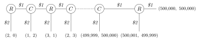
Unlike the Prisoner’s Dilemma, this is a game of perfect information: the players move one at a time, and each knows, when it is his or her turn, everything that has happened so far. And it is a game that rewards patience handsomely. If both players keep going across, they split the pile evenly, and each walks away with half a million dollars. If Row goes down at the very first move, he gets $2 and Column gets nothing.
Now apply backwards induction. At the last move, move , there are two dollars left and it is Row’s turn. Going down gets him both, for a total of $500,001, whereas going across gets him one, for a total of $500,000 (leaving the last dollar to Column); so, if he is rational, he goes down. At move , Column knows this, so she knows that if she goes across Row will go down, leaving her with $499,999; going down now gets her $500,000, so she goes down. At move , Row knows that if he goes across Column will go down, leaving him with $499,999, whereas going down now gets him $500,000; so he goes down. And so on: at every move, the player whose turn it is gets two dollars by going down, but only one by going across if the other player then goes down. At the very first move, then, Row goes down, and the game ends with Row getting $2 and Column nothing, when each of them could have had half a million dollars. Backwards induction tells us that the game will end as soon as it begins.
10.8.4 The role of common knowledge
Both backwards induction arguments rely on the players’ knowing a great deal about each other, and it is worth being precise about how much. Take the centipede game. Row’s going down at the last move requires only that he be rational. Column’s going down at the second-to-last move requires, in addition, that she know that Row is rational. Row’s going down at the third-to-last move requires that he know that Column is rational and that he know that Column knows that he is rational. Each move further back requires one more layer, so that Row’s going down at the very first move requires layers: Row must know that Column knows that Row knows that Column knows … ( “knows” in all) … that the player who moves last is rational. In general, in a centipede game with moves the argument for going down at the first move needs layers of knowledge, and in the hundred-round Prisoner’s Dilemma the argument for confessing in round needs . This is just the phenomenon we saw in our discussion of iterated deletion of dominated strategies: each step of the reasoning requires one more layer of knowledge than the one before. The assumption that rationality is common knowledge (Definition 10.3) delivers all the layers at once.
But now suppose that just one of those layers fails, however deep it is. In the hundred-round Prisoner’s Dilemma, for instance, suppose that the first ninety-eight layers hold, but the ninety-ninth does not. Then the backwards induction argument for confessing in round breaks down: Row can no longer be sure that Column will confess in round whatever happens in round , and so, for all Row knows, staying silent in round may buy him Column’s silence later on. And because the stakes in these games are so lopsided, it does not take much doubt to make cooperation rational. In the centipede game, suppose Row thinks that there is a probability that Column is the kind of player who will keep going across as long as Row does, and a probability that she will go down at the first opportunity. If Row goes down at once, he gets $2. If he goes across, then with probability Column goes down at the second move, leaving Row with $1; and with probability the game continues until Row goes down at the last move, leaving him with $500,001. Going across has the higher expected utility as long as Any chance greater than one in half a million that Column will cooperate is enough to make going across rational for Row; and the same kind of reasoning applies at later moves, and to staying silent in the early rounds of a repeated Prisoner’s Dilemma. So the distressing conclusions of the backwards induction arguments follow only if the players’ rationality is known to a very great depth, and even a very high number of layers is not enough if it falls short of what the argument needs: ninety-eight layers will not do in a hundred-round Prisoner’s Dilemma, and will not do in our centipede game. Experiments fit this picture: when people play centipede games in the laboratory, very few of them go down at the first move; most go across for a while, and go down only as the end of the game approaches.
There is a final twist. Suppose that Row, despite the backwards induction argument, goes across at the first move, and Column finds herself at the second node. Column now knows something that, if rationality were common knowledge, could not have happened: Row has gone across. How should she reason from here? Should she conclude that Row is not rational after all, or that Row does not know that she is rational, or that Row is trying to signal something? Whatever she concludes, it seems that she can no longer take for granted the very assumptions on which the backwards induction argument relied. Philosophers and game theorists continue to disagree about how to reason in such situations, and so about whether common knowledge of rationality really does support the backwards induction solution of games like the centipede.
Exercises
Strategies, trees, and matrices. In the game below, Row first chooses Up or Down. Column sees what Row chose, and then chooses Left or Right. At each leaf, Row’s utility is listed first and Column’s second.
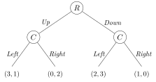
Column has four strategies (Definition 10.2). List them. (Remember that a strategy for Column must say what she would do if Row played Up and what she would do if Row played Down.)
Write down the matrix of the game, with Row’s two strategies as rows and Column’s four strategies as columns.
Find all the pure Nash equilibria of the game by starring best responses.
Now suppose that Column does not see what Row chose before making her own choice. Draw the tree for this new game, write down its matrix, and find its pure Nash equilibria, if any. What difference does it make that Column can see Row’s choice?
Show solution
Column’s strategies are LL, LR, RL, RR, where each letter is the response to Up and then to Down. Pairs are (Row, Column):
LL LR RL RR Up Down The unique Nash equilibrium is (Down, RL), with outcome . In the simultaneous version (leaves , , , ) there is no pure-strategy equilibrium. So Column’s observing Row’s move makes the difference: with observation the game has exactly one equilibrium, ; without it, none.
From matrices to trees. Draw a tree for the Park or Movies game (Table 10.4), drawing Row as moving first. Then draw a second tree for the same game, this time drawing Column as moving first. Explain why the two trees represent the very same game.
Show solution
Two trees, with leaves equal to , one for each player moving first. In the tree where Row moves first, Column’s two decision nodes are joined by a dotted line (one information set), since Column cannot see Row’s move:
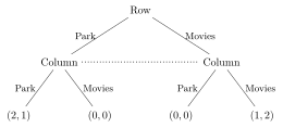
For the other tree, Column moves first and Row’s nodes are joined, with the leaves written as in the same pattern: Park–Park , Park–Movies , Movies–Park , Movies–Movies . The matrix does not encode the order of play; the trees do, and they also show what each player can observe.
Zero-sum games. For each of the following games, say whether it is zero-sum. If it is, rewrite its matrix with Row’s utilities only.
For game (c), show that a positive linear transformation of Column’s utilities (Definition 8.1) turns it into a zero-sum game. Why is this transformation legitimate?
Show solution
(a) Zero-sum; the Row-only matrix is . (b) Not zero-sum. (c) Constant-sum with total . Utilities are fixed only up to a positive linear transformation, so subtracting from Column’s utilities (, ) changes neither choices nor equilibria; it gives the Row-only matrix .
Iterated deletion. Solve each of the following games by iterated deletion of strongly dominated strategies. At each step, say which strategy you delete and which strategy dominates it. Game (a) is zero-sum and is written, as usual, with Row’s utilities only.
Practice in the Games Lab Delete the strongly dominated strategies yourself, and the lab checks each step.
Practice in the Games Lab Delete the strongly dominated strategies yourself, and the lab checks each step.
For game (a), say how many layers of knowledge about the other player’s rationality each step of the deletion requires.
Show solution
(a) Delete R3 (strictly dominated by R2), then C1 (by C2), then R1 (by R2), then C3 (by C2). What remains is (R2, C2), with value . Dominance is judged in the reduced game, so the deletions need prior layers. (b) Delete C2 (by C1), R2 (by R1), C3 (by C1), R3 (by R1). What remains is (R1, C1) .
Starring best responses. Find all the pure Nash equilibria of each of the following games by starring best responses, or show that there are none. For game (c), also find all the Pareto optimal outcomes (Definition 10.9), and say whether the Nash equilibrium is one of them.
Practice in the Games Lab Find the Nash equilibria yourself, and the lab checks your answer.
Practice in the Games Lab Find the Nash equilibria yourself, and the lab checks your answer.
Practice in the Games Lab Find the Nash equilibria yourself, and the lab checks your answer.
Practice in the Games Lab Find the Pareto optimal outcomes yourself, and the lab checks your answer.
Show solution
(a) Two equilibria: (R2, C1) and (R3, C3) . (b) None. (c) A unique equilibrium, (R3, C2) . The Pareto optimal outcomes in (c) are (R1, C4) , (R2, C4) and (R3, C2) , so the equilibrium is Pareto optimal.
Saddle points. Each of the following zero-sum games is written with Row’s utilities only. For each one, write down the minimum of each row and the maximum of each column, find the maximin and the minimax, and find all the saddle points, if any. For the game with more than one saddle point, check that they all have the same value.
Practice in the Games Lab Find the maximin, the minimax and the saddle points yourself, and the lab checks your answer.
Practice in the Games Lab Find the maximin, the minimax and the saddle points yourself, and the lab checks your answer.
Practice in the Games Lab Find the maximin, the minimax and the saddle points yourself, and the lab checks your answer.
Show solution
(a) Maximin minimax ; one saddle point, (R3, C4). (b) Maximin minimax ; no saddle point. (c) Maximin minimax ; saddle points (R1, C1) and (R1, C2), both of value .
Weak dominance. Consider the following game.
Practice in the Games Lab Find the Nash equilibria yourself, and the lab checks your answer.
Find all the pure Nash equilibria of the game.
Show that is weakly, but not strongly, dominated.
Delete , and keep deleting weakly dominated strategies until no more can be deleted. What is left? Which Nash equilibrium of the original game has been lost along the way?
Show solution
The Nash equilibria are (R1, C2) and (R2, C1) . Column’s C3 weakly (not strongly) dominates C2. Deleting C2, then R1 (now weakly dominated by R2), then C3 leaves only (R2, C1). The equilibrium lost by iterated deletion of weakly dominated strategies is (R1, C2).
Prisoner’s Dilemmas and their relatives. For each of the following games, answer these questions: Does either player have a dominant strategy? What are the pure Nash equilibria? Which outcomes are Pareto optimal? Is the game a Prisoner’s Dilemma?
Practice in the Games Lab Find the Nash equilibria yourself, and the lab checks your answer.
Practice in the Games Lab Find the Pareto optimal outcomes yourself, and the lab checks your answer.
Practice in the Games Lab Find the Nash equilibria yourself, and the lab checks your answer.
Practice in the Games Lab Find the Pareto optimal outcomes yourself, and the lab checks your answer.
Practice in the Games Lab Find the Nash equilibria yourself, and the lab checks your answer.
Practice in the Games Lab Find the Pareto optimal outcomes yourself, and the lab checks your answer.
Show solution
(a) Prisoner’s dilemma: R2 and C2 are dominant, the unique equilibrium is , and every outcome except is Pareto optimal. (b) Stag hunt: no dominant strategies; equilibria (R1, C1) and (R2, C2); only is Pareto optimal. Not a prisoner’s dilemma. (c) R1 and C1 are dominant; the equilibrium is , the only Pareto optimal outcome. Not a prisoner’s dilemma.
Playing with a twin. You are playing the Prisoner’s Dilemma of Table 10.20 against your twin, and you are confident that, whatever you decide to do, your twin will decide the same.
Compute the conditional expected utility of staying silent and of confessing. Which option does MCEU recommend? Which option does dominance reasoning recommend?
Let be your confidence that your twin will decide as you do. For which values of does MCEU recommend staying silent?
Show solution
With : and , so MCEU says to stay silent while dominance says to confess. In general and , so Silent is recommended exactly when .
A short centipede. Consider the centipede game of Figure 10.4, but with a pile of only six one-dollar bills.
Draw the tree of the game, listing each player’s total winnings at each leaf.
Use backwards induction to find out what rational players would do. What are the players’ winnings?
How many layers of knowledge of rationality does the backwards induction argument require for Row’s first move?
Suppose Row thinks that there is a probability that Column is the kind of player who will keep going across as long as Row does, and a probability that she will go down at her first opportunity. For which values of is going across at the first move better for Row than going down?
Show solution
(a) The tree alternates Row, Column, Row, Column, Row; at each node the mover chooses down (ending the game) or across. The leaves reached by down are, in order, , , , , , and the final across gives . (b) By backwards induction, Row goes down at the first move, giving . (c) Four layers of knowledge are needed. (d) Going across is better iff , i.e. .
Conceptual questions.
A teacher tells each of her students, in private, that tomorrow’s exam has been cancelled. Is the cancellation mutually known among the students? Is it common knowledge (Definition 10.3)? What could the teacher do to make it common knowledge?
A mother plays chess against her young son, and wants him to win. Two grandmasters play chess against each other, and each wants to win. Explain why, according to game theory, these are not the same game, even though the rules of chess are the same in both cases.
Explain why the backwards induction argument for confessing in every round of a repeated Prisoner’s Dilemma cannot get started if the players do not know how many rounds they will play.
Describe a situation from everyday life, other than those mentioned in the chapter, that has the structure of a Prisoner’s Dilemma. Then describe a law, contract, or social norm that could change the payoffs so that the people involved are no longer in a Prisoner’s Dilemma.
Show solution
(a) Mutual knowledge, yes; common knowledge, no; the announcement should be public. (b) Games are individuated by their utilities, not by their outward description: the mother’s goal is that her son win, so her utilities differ from what the rules alone suggest and the game is a different one. (c) Backwards induction starts from the last move; if there is no last round (or the players do not know when it is), there is no starting point for the induction, and cooperation can be sustained. (d) An everyday prisoner’s dilemma together with a law, contract or norm that changes the payoffs, so that the strategy that was dominated becomes unattractive.