PHIL 109 · Introduction to Formal Reasoning and Decision Making

6 Bayesianism

6.1 The lottery paradox: beliefs and credences

In order to win Italy’s “SuperEnalotto” lottery, one has to correctly predict 6 numbers out of a pool of 90 (order doesn’t matter). There are 622,614,630 ways of picking 6 numbers out of 90.¹ Consider all those possible entries in the lottery, one by one, and suppose that for each one we ask: is it going to win? If forced to answer “Yes” or “No”, I would say “No”. And it is also natural to think that buying an entry in the SuperEnalotto is a waste of money because one’s entry is not going to win. This suggests that we believe, of any given entry, that it is not going to win. Fix some way of numbering the possible entries (for instance, order the numbers from smallest to largest in each entry, and order the entries from smallest to largest resulting number). Let “1” represent the proposition ticket number 1 will win, “2” the proposition ticket number 2 will win; in general, let $n$ represent the proposition ticket number n will win. If we believe, of each ticket, that it will not win, then we believe all of these propositions:

$\neg 1$
$\neg 2$
$\ldots$
$\neg 622{,}614{,}630$

But we also believe that one of those tickets will win. That is to say, we believe the following disjunction:

$1 \lor 2 \lor \ldots \lor 622{,}614{,}630$

Those 622,614,631 beliefs of ours are contradictory. This is easy to see: if each ticket is a loser (as our first 622,614,630 beliefs say they are), then no ticket is a winner (contradicting our 622,614,631st belief). Apparently, the intuitive reaction to what we should believe about a lottery lands us in contradiction.

Some think that the way out of this contradiction is to realize that not all of our opinions are all-or-nothing. The lottery paradox arises because we are forced to say whether we believe that a ticket will win or not. But perhaps our opinion is not well represented by a “Yes” or “No” answer to that question, but rather by a graded answer: we are pretty sure that each ticket is going to lose, but we are not certain. In fact, we can even quantify how sure we are, of each ticket, that it is going to lose: we are $1 - \frac{1}{622{,}614{,}630}$ sure, of each ticket, that it is going to lose—and $\frac{1}{622{,}614{,}630}$ sure that it is going to win. These degrees of beliefs are sometimes called credences. Once we think of the SuperEnalotto in terms of credences instead of all-or-nothing beliefs, the paradox disappears. Notice that $\{1, 2, \ldots, 622{,}614{,}630\}$ is a set of pairwise mutually exclusive propositions (one ticket’s winning is incompatible with any other ticket’s winning: we stipulate that the possible worlds under consideration are just those in which exactly one ticket wins). Therefore, by Theorem 5.9, the probability that any one of a number of tickets will win is the sum of the probability that each one of them will win. Therefore, the probability that some ticket or other will win is 1! If we align our credences with these (known to us) probabilities, then we can have, for each ticket, an extremely low credence that it will win, while at the same time having credence 1 that some ticket will win.

Needless to say, not all philosophers are convinced by the above argument that credences are psychologically real. But in what follows we proceed with the hypothesis that they are, and see where that leads us.

6.2 Bayesianism

Our credence-first treatment of the lottery paradox had us align our credences with the known probabilities, and thus our credences themselves were probabilities: they satisfied Non-negativity, Normality, and Additivity. Some people believe that this should always be the case: they think that, in order to be rational, our credences should satisfy the probability axioms. Because it applies to our credences at a time, we will call this the synchronic norm for credences:

The synchronic norm for credences establishes relationships between the credences we have in different propositions at a time. For instance, our credences in a proposition and its negation cannot float free from each other—one must be 1 $-$ the other.

But we are not just interested in how our credences relate to each other at a single time, we also want to know how to change our credences once we acquire new evidence. To simplify discussion, let us concentrate on just two propositions $H$ and $E$. Let $E$ = Shaun studies hard for the exam, and $H$ = Shaun passes the exam. How should we fill-in the stochastic truth-table for these two propositions? To do so we need to assign credences not just to the individual propositions $H$ and $E$, but to each of the four possible worlds determined by them—to each row of the stochastic truth-table. Thus, let us suppose that we are 50-50 on whether Shaun will pass the exam, when that proposition is considered independently of whether or not he studies hard, and let us also suppose that we are 50-50 on whether or not he will study hard. However, we are much more confident that he will pass conditional on his studying than otherwise—let us say, we think the possible world where he passes and studies hard is 9 times more likely than the possible world where he passes but doesn’t study hard. In that case, we will fill-in the stochastic truth-table as follows (notice that we rename the $\Prb$ column $\Cr$, because we are thinking of credences now):

Try it in the Probability Lab Step through this stochastic truth table. The lab names the sentence letters P, Q, ...: here H is P, E is Q.

Notice that, as we know, unconditional probabilities determine conditional probabilities. In particular, we can add a column for credences conditional on $E$:

Try it in the Probability Lab Step through this stochastic truth table, with its conditional column. The lab names the sentence letters P, Q, ...: here H is P, E is Q.

As stipulated, our credence that Shaun will pass the test, conditional on his studying hard, is 0.9, whereas our credence that he will pass conditional on his not studying is only 0.1 (the world where he passes without studying has credence $\sfrac{1}{20}$, which is one tenth of our credence of $\sfrac{1}{2}$ that he does not study). Notice that all of these credences—conditional and unconditional—do not commit us one way or the other on either whether Shaun will pass the exam or whether he will study—we are still 50-50 on those propositions.

But now suppose that we learn that Shaun did study hard. How should we change our credences? Should we still be 50-50 on whether he will pass? Well, should we still be 50-50 on whether he studied hard? Clearly not: we learned that he did study hard, so we should now have credence 1 that he did and credence 0 that he did not. And how should that affect our credence that he will pass? If you think it should make us more confident that he will pass, you are not alone. Indeed, many philosophers have argued that we should now be 90% confident that he will pass the exam. Those philosophers adhere to the following diachronic norm for credences:

We have to be very careful in distinguishing the definition of conditional probability from the diachronic norm for credences. The former is just stipulated to be a ratio of your unconditional credences at a time, whereas the latter is a norm for how your credences should change over time. Of course, the diachronic norm for credences is intimately related to conditional probabilities, for it commands you to change your credences by appealing to your old conditional credences—but they are still two very different things. For instance, many would reject the diachronic norm for credences, but that doesn’t commit them to denying the existence of conditional probabilities.

“Bayesianism” will be our name for the view that adopts both the synchronic and the diachronic norms for credences. In order to explain the name, we need to introduce one more theorem about conditional probabilities:

The theorem is named after Thomas Bayes, an eighteenth-century English statistician, philosopher, and Presbyterian minister who first formulated a special case of it. It relates the conditional probability of, e.g., $H$ given $E$, to the converse conditional probability of $E$ given $H$. The theorem should not be confused either with the definition of conditional probability or with the diachronic norm for credences. Its importance, however, is related to the diachronic norm for credences, because the information we have often makes it easier to calculate conditional probabilities by appealing to Bayes’ theorem rather than the definition of conditional probability—and, of course, conditional probabilities need to be calculated in order to apply the diachronic norm for credences.

The quantities in Bayes’ theorem have traditional names. $\Prb(\varphi \given \psi)$ is called the posterior probability, $\Prb(\varphi)$ and $\Prb(\psi)$ the prior probabilities, and $\Prb(\psi \given \varphi)$ the likelihood (of the hypothesis $\varphi$, relative to the evidence $\psi$). Let us apply the theorem to our example about Shaun and his exam:

$$\Cr(H \given E) = \frac{\Cr(E \given H) \times \Cr(H)}{\Cr(E)} = \frac{\frac{9}{10} \times \frac{1}{2}}{\frac{1}{2}} = \frac{9}{10}$$

$\Cr(H \given E)$ is called the posterior probability because it is the credence you will have in $H$ after conditionalizing on $E$, and $\Cr(H)$ is called the prior probability because it is credence you have in $H$ before conditionalizing on $E$. Why $\Cr(E \given H)$ is called the likelihood is a mystery.²

There is another form of Bayes’ theorem that will be useful as well. In order to state it, we need to prove another theorem:

Theorem 6.4 tells us that the probability of any proposition is an average of its probabilities conditional on any other proposition and its negation, weighted by the probabilities of that other proposition and its negation. This means that we can re-write the denominator in Bayes’ theorem (notice that when we use Theorem 6.4 in the theorem below we switch $\varphi$ and $\psi$, to match Theorem 6.3):

This version of Bayes’ theorem is useful because we will sometimes not know what the probability of the evidence is directly, but we will know the likelihood of the evidence given both the hypothesis and its negation.

Let us exemplify with Leona. Recall the argument from Chapter 4:

• (1) Leona has a heavy, shaggy coat, a long bushy tail, and large tufted ears.
• (2) Most Maine Coons have those characteristics, and relatively few cats which are not Maine Coons do.
• $\therefore$ Leona is a Maine Coon.

Is that argument good? It is not valid, but we know that not all good arguments are valid. Let us try to formalize it and apply our probability tools to see how good it is. We start with a dictionary. The first premise and the conclusion are easy to symbolize:

Dictionary:

$L$ = Leona has a heavy, shaggy coat, a long bushy tail, and large tufted ears.
$M$ = Leona is a Maine Coon.

But how should we symbolize the second premise? To begin with, we’ll do well to separate its two components: most Maine coons have a heavy, shaggy coat, a long bushy tail, and large tufted ears; most non-Maine Coon cats do not. We do not want to translate each of these components as a new atomic proposition, because that way we would lose important information. Rather, we want to see how to connect that second premise to the other one and the conclusion. Intuitively, the idea is clear: any cat’s being a Maine Coon must raise the probability that it has the characteristic Leona has, and any cat’s not being a Maine Coon must lower it. Let us suppose that $\Cr_{old}(L \given M) = \frac{9}{10}$ and that $\Cr_{old}(L \given \neg M) = \frac{1}{5}$. Now we are told that $L$ is true. How should we update our credences? According to the diachronic norm for credences, we should do the following:

$$\Cr_{new}(M) = \Cr_{old}(M \given L)$$

We can now try to apply Bayes’ theorem to this problem:

$$\Cr_{old}(M \given L) = \frac{\Cr_{old}(L \given M) \times \Cr_{old}(M)}{\Cr_{old}(L)} = \frac{\frac{9}{10} \times \Cr_{old}(M)}{\Cr_{old}(L)}$$

That wasn’t too much progress, because we are left with two unknowns still. Switching to the LTP version of Bayes’ theorem helps a lot:

$$\begin{aligned} \Cr_{old}(M \given L) &= \frac{\Cr_{old}(L \given M) \times \Cr_{old}(M)}{\Cr_{old}(L \given M) \times \Cr_{old}(M) + \Cr_{old}(L \given \neg M) \times \Cr_{old}(\neg M)} \\[8pt] &= \frac{\frac{9}{10} \times \Cr_{old}(M)}{\frac{9}{10} \times \Cr_{old}(M) + \frac{2}{10} \times \Cr_{old}(\neg M)} \end{aligned}$$

But we still have two unknowns: $\Cr_{old}(M)$ and $\Cr_{old}(\neg M)$. Well, actually it’s just one unknown, because we know by Theorem 5.5 that one of them can be derived from the other. So, what should $\Cr(M)$ be—that is to say, what should our credence that Leona is a Maine Coon be before we know anything about her? Well, remember the other fact we mentioned about Maine Coons: that they make up about 10% of all cats. If we guide our priors by this, then $\Cr(M) = \frac{1}{10}$ and $\Cr(\neg M) = \frac{9}{10}$. Plugging in those numbers:

$$\begin{aligned} \Cr_{old}(M \given L) &= \frac{\frac{9}{10} \times \frac{1}{10}}{\frac{9}{10} \times \frac{1}{10} + \frac{2}{10} \times \frac{9}{10}} \\[8pt] &= \frac{\frac{9}{100}}{\frac{9}{100} + \frac{18}{100}} \\[8pt] &= \frac{\frac{9}{100}}{\frac{27}{100}} \\[8pt] &= \frac{9}{27} \\[8pt] &= \frac{1}{3} \end{aligned}$$

And so $\Cr_{new}(M) = \frac{1}{3}$. Which means two things: first, the fact that Leona has Maine Coon-ish characteristics is indeed good evidence that she is a Maine Coon—we went from $\Cr_{old}(M) = \frac{1}{10}$ to $\Cr_{new}(M) = \frac{1}{3}$, which means that our credence that Leona is a Maine Coon more than tripled; but second, we still think that it is twice as likely that Leona is not a Maine Coon. How could that be? Relatedly, how could it be that having Maine Coon-ish characteristics is such good evidence for being a Maine Coon while at the same time most cats with those characteristics are not Maine Coons? The answer is in the priors. There are many more cats that are not Maine Coons than there are cats that are. Thus, suppose that we concentrate on a random population of 100 cats. 10 of them will be Maine Coons, and of those 9 will have Maine Coon-ish characteristics. Meanwhile, 90 of them will not be Maine Coons, and 18 of those will have Maine Coon-ish features. Thus, if a randomly selected cat has Maine Coon-ish features, it is twice as likely to not be a Maine Coon as to be one–even when those features are had by 90% of Maine Coons and only by 20% of cats that are not Maine Coons.

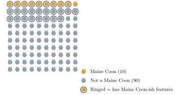
Try it in the Probability Lab Follow Bayes' theorem step by step in the lab. The lab calls the hypothesis H and the evidence E: here M is H and L is E.

The moral is: don’t conclude that a hypothesis $H$ is true just because you have some evidence $E$ which is predicted very well by the hypothesis—i.e., $\Prb(E \given H)$ is very high. How strongly $E$ favors $H$ depends not on $\Prb(E \given H)$ alone but on how it compares with $\Prb(E \given \neg H)$, that is, on the likelihood ratio $\frac{\Prb(E \given H)}{\Prb(E \given \neg H)}$. (In Leona’s case the ratio is $\frac{9/10}{1/5} = \frac{9}{2}$: her features are four and a half times as likely if she is a Maine Coon as if she is not.) The likelihood ratio is one of the factors that, according to Bayes’ theorem, determine the posterior—$\Prb(H \given E)$. But the other important factor is the prior $\Prb(H)$. This prior is also sometimes called the “base rate”, and concluding that $\Prb(H \given E)$ must be high just because $\Prb(E \given H)$ is high is sometimes called the fallacy of base rate neglect.

6.3 Eikosograms

So far we have reasoned about probabilities entirely algebraically—writing down axioms, deriving theorems, and grinding through fractions like the ones in Leona’s case. That is one way to get the right answer, but it is easy to lose the forest for the trees: it is not always obvious why $\Prb(M \given L) = \sfrac{1}{3}$ feels surprising, or why it should not. In this section we introduce a picture—the eikosogram—that lets us see probabilities as areas, and that makes facts like Leona’s fairly small posterior almost obvious to the eye.

An eikosogram is a square of area 1 that allows us to compare the probabilities of each possible world determined by two propositions $\varphi$ and $\psi$. The square is divided into a left strip and a right strip by a vertical line. We then divide each of the strips into a top and bottom part. The lines dividing the left and right strip need not match up with each other. The four resulting rectangles—bottom-left, top-left, bottom-right, and top-right—correspond to $\varphi \land \psi$, $\varphi \land \neg \psi$, $\neg \varphi \land \psi$, and $\neg \varphi \land \neg \psi$, respectively. The probability of each of these four molecular propositions (which, you’ll notice, are the rows of the corresponding truth-tables) is the area of the corresponding rectangle. The width of the left strip corresponds to $\Prb(\varphi)$ and that of the right strip to $\Prb(\neg \varphi)$. $\Prb(\psi)$ corresponds to the (possibly irregular) shape that is the combination of the two bottom rectangles. The height of the bottom-left rectangle is $\Prb(\psi \given \varphi)$, and the height of the bottom-right rectangle is $\Prb(\psi \given \neg \varphi)$.

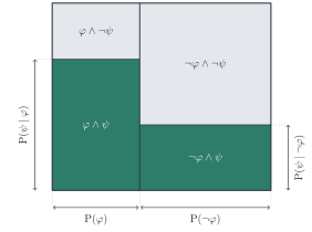
That is why eikosograms are useful: every probability we might want—an unconditional probability like $\Prb(\varphi)$, a conjunction like $\Prb(\varphi \land \psi)$, even a conditional probability like $\Prb(\psi \given \varphi)$, which is just the height of a strip—can be read directly off the diagram, as a length or an area.

Let us return to Leona. Recall that $\Prb(M) = \sfrac{1}{10}$, $\Prb(L \given M) = \sfrac{9}{10}$, and $\Prb(L \given \neg M) = \sfrac{2}{10}$. Figure 6.3 shows the resulting eikosogram.

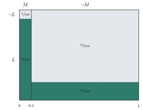
The picture makes both parts of our earlier result vivid at once. First, the dark (“has characteristics”) rectangle in the $M$ strip takes up nearly all of that strip’s height—because $\Prb(L \given M) = \sfrac{9}{10}$ is large, having the characteristics really is good evidence of being a Maine Coon. Second, the $M$ strip itself is thin: because $\Prb(M) = \sfrac{1}{10}$ is small, even a tall dark rectangle within it covers only a small area, $\sfrac{9}{100}$. Meanwhile the dark rectangle in the much wider $\neg M$ strip, though comparatively short, covers a bigger area, $\sfrac{18}{100}$, simply because it has so much more width to work with. Geometrically, Bayes’ theorem is nothing more than comparing one dark rectangle to the sum of both.

6.4 Hume on miracles

In a very famous passage of his Enquiry Concerning Human Understanding, David Hume writes:

No testimony is sufficient to establish a miracle, unless the testimony be of such a kind, that its falsehood would be more miraculous, than the fact, which it endeavours to establish. (...) When any one tells me, that he saw a dead man restored to life, I immediately consider with myself, whether it be more probable, that this person should either deceive or be deceived, or that the fact, which he relates, should really have happened. I weigh the one miracle against the other; and according to the superiority, which I discover, I pronounce my decision, and always reject the greater miracle. If the falsehood of his testimony would be more miraculous, than the event which he relates; then, and not till then, can he pretend to command my belief or opinion.

In this section we will analyze this passage using what we’ve learned in this part.

A miracle, for Hume, is a violation of a law of nature. And Hume’s conception of a law of nature is a regularity that has been found by unexceptional experience. For instance, a man’s being resurrected would be a miracle. It’s important to note that Hume does not think that miracles are impossible. A miracle is something that goes against all of our vast experience so far, but is not a contradiction.

Hume’s argument seems to be the following:

• (1) If testimony is sufficient to establish a miracle, then it’s less likely that the testimony is false than that the miracle occurred.
• (2) It is always more likely that the testimony is false than that a miracle occurred.
• $\therefore$ No testimony is sufficient to establish a miracle.

Let us start our analysis with a dictionary. Which atomic propositions are used in Hume’s argument? It helps to start with the conclusion: that no testimony is sufficient to establish a miracle. This is clearly the negation that testimony is (sometimes) sufficient to establish a miracle. How could we symbolize in PL that proposition? One possibility is as a conditional: if someone testifies that a miracle occurred, then a miracle occurred. The first premise then says that if a miracle can ever be established by testimony, then it’s less likely that the testimony is false than that the miracle occurred. Our dictionary, then, can be the following:

$T$ = Someone testifies that a miracle occurred.

$M$ = A miracle occurred.

$F$ = It’s less likely that the testimony is false than that a miracle occurred.

We can then reconstruct the argument as follows:

• (1) $(T \to M) \to F$
• (2) $\neg F$
• $\therefore$ $\neg M$

The argument is valid, as you can verify by constructing its truth-table. Now, what about the premises? Let’s start with the first one:

If testimony is sufficient to establish a miracle, then it’s less likely that the testimony is false than that the miracle occurred.

What does it mean to say that testimony is sufficient to establish a miracle? We can assume that if our credence that a miracle has happened is less than 50%, then the miracle is not established, so let us say that testimony $T$ establishes a miracle $M$ (for us) just in case our degree of belief in $M$ given $T$ is at least 50%:

A miracle has been established $=$ $\Cr_{old}(M \given T) \geq 0.5$

Then we receive as evidence the testimony $T$ that the miracle in question has occurred. What should our degree of belief in $M$ be now? If we are Bayesians, it should be: $$\tag{1} \Cr_{new}(M) = \Cr_{old}(M \given T) = \frac{\Cr_{old}(T \given M) \times \Cr_{old}(M)}{\Cr_{old}(T)}$$ In the same way, our credence that no miracle has occurred after hearing testimony that it has is given by: $$\tag{2} \Cr_{new}(\neg M) = \Cr_{old}(\neg M \given T) = \frac{\Cr_{old}(T \given \neg M) \times \Cr_{old}(\neg M)}{\Cr_{old}(T)}$$ Dividing (1) by (2), the unknown $\Cr_{old}(T)$ cancels out, which means that the odds of our credence that a miracle has occurred to our credence that it has not (after hearing testimony in its favor) are given by the following:³ $$\tag{3} \frac{\Cr_{old}(M \given T)}{\Cr_{old}(\neg M \given T)} = \frac{\Cr_{old}(T \given M)}{\Cr_{old}(T \given \neg M)} \times \frac{\Cr_{old}(M)}{\Cr_{old}(\neg M)}$$ Since $\Cr_{new}$ is a probability function, Theorem 5.5 gives $\Cr_{new}(\neg M) = 1 - \Cr_{new}(M)$, and so $\Cr_{old}(\neg M \given T) = 1 - \Cr_{old}(M \given T)$: $$\tag{4} \Cr_{old}(M \given T) \geq 0.5 \quad\text{iff}\quad \frac{\Cr_{old}(M \given T)}{\Cr_{old}(\neg M \given T)} \geq 1$$ Now, from (3) and (4) it follows that: $$\tag{5} \Cr_{old}(M \given T) \geq 0.5 \quad\text{iff}\quad \frac{\Cr_{old}(T \given M)}{\Cr_{old}(T \given \neg M)} \times \frac{\Cr_{old}(M)}{\Cr_{old}(\neg M)} \geq 1$$ Rearranging (5): $$\tag{6} \Cr_{old}(M \given T) \geq 0.5 \quad\text{iff}\quad \frac{\Cr_{old}(M)}{\Cr_{old}(\neg M)} \geq \frac{\Cr_{old}(T \given \neg M)}{\Cr_{old}(T \given M)}$$ Equivalently: $$\tag{7} \Cr_{old}(M \given T) \geq 0.5 \quad\text{iff}\quad \Cr_{old}(T \given \neg M) \leq \Cr_{old}(T \given M) \cdot \frac{\Cr_{old}(M)}{\Cr_{old}(\neg M)}$$ If we assume that the testifier will definitely testify to the miracle if he experiences it (i.e., that $\Cr_{old}(T \given M) \approx 1$—notice that this assumption is friendly to the believer in miracles), we have that: $$\tag{8} \Cr_{old}(M \given T) \geq 0.5 \quad\text{iff}\quad \Cr_{old}(T \given \neg M) \lesssim \frac{\Cr_{old}(M)}{\Cr_{old}(\neg M)}$$ If we assume with Hume that $\Cr_{old}(M) \approx 0$ (but positive!), then $\frac{\Cr_{old}(M)}{\Cr_{old}(\neg M)} \approx \Cr_{old}(M)$, and so: $$\tag{9} \Cr_{old}(M \given T) \geq 0.5 \quad\text{iff}\quad \Cr_{old}(T \given \neg M) \lesssim \Cr_{old}(M)$$ And (9) can be seen as a probabilistic reconstruction of Hume’s premise 1: a testimony can establish a miracle just in case it is less likely that such testimony would be given falsely—that is, given even though no miracle occurred, $\Cr_{old}(T \given \neg M)$—than that the miracle occurred. (Notice that this is not the probability that the testimony is false, $\Cr_{old}(\neg M \given T)$: that is the very posterior we are trying to compute.) Call (9) Hume’s test. So the test itself is (a strengthening of) premise 1, and Hume’s contention that no testimony passes that test (i.e., that the falsity of a testimony is always more likely than the occurrence of a miracle) is his premise 2. So, is his premise 2 true? Let us try to put some numbers into the probabilities.

Let us suppose that the odds against a miracle are 10,000 to 1—a very liberal view of miracles that is not at all friendly to Hume. In that case, $\Cr_{old}(M) = \frac{1}{10{,}001}$, and, correspondingly, $\Cr_{old}(\neg M) = \frac{10{,}000}{10{,}001}$. Let us also assume that if a miracle did in fact occur, then it will for sure be testified to: $\Cr_{old}(T \given M) = 1$. Hume’s crucial point is that, nevertheless, there will be some false testimonies—due to intentional misleadingness, or self-deception, or whatever. So let us suppose that testimony to a miracle is rarely produced when no miracle has occurred: in 1 out of every 100 cases in which there is no miracle, there is nonetheless testimony that there was one: $\Cr_{old}(T \given \neg M) = \frac{1}{100}$.

Now we compute the posterior using the LTP version of Bayes’ theorem: $$\begin{aligned} \Cr_{new}(M) &= \Cr_{old}(M \given T)\\ &= \frac{\Cr_{old}(T \given M) \times \Cr_{old}(M)}{\Cr_{old}(T \given M) \times \Cr_{old}(M) + \Cr_{old}(T \given \neg M) \times \Cr_{old}(\neg M)}\\ &= \frac{1 \times \frac{1}{10{,}001}}{1 \times \frac{1}{10{,}001} + \frac{1}{100} \times \frac{10{,}000}{10{,}001}}\\ &= \frac{\frac{1}{10{,}001}}{\frac{1}{10{,}001} + \frac{100}{10{,}001}}\\ &= \frac{1}{101}\\ &\approx 0.00990099 \; (=0.990099\%). \end{aligned}$$

So, even with assumptions that are friendly to the existence of miracles and the veracity of testifiers, Hume’s point seems to stand: our credence in a miracle on the basis of testimony for it should be less than 0.01. The eikosogram would look something like this (although we cannot really represent how thin the left rectangle would have to be and keep it visible):

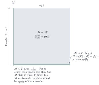
But what if what we receive as evidence is not just a single testimony, but several? A crucial point here is whether these testifiers give us independent evidence or not. If a second testifier is just repeating what the first one says because she believes him, that should not add any evidence in favor of the miracle. Let us suppose, then, that we receive two testimonies $T_1$ and $T_2$, and that the testifiers are conditionally independent given $M$ and given $\neg M$: $$\begin{aligned} \Cr_{old}(T_1 \land T_2 \given M) &= \Cr_{old}(T_1 \given M) \times \Cr_{old}(T_2 \given M),\\ \Cr_{old}(T_1 \land T_2 \given \neg M) &= \Cr_{old}(T_1 \given \neg M) \times \Cr_{old}(T_2 \given \neg M). \end{aligned}$$ Assume, as before, that $\Cr_{old}(T_1 \given M) = \Cr_{old}(T_2 \given M) = 1$ and that $\Cr_{old}(T_1 \given \neg M) = \Cr_{old}(T_2 \given \neg M) = \frac{1}{100}$. Then: $$\begin{aligned} \Cr_{old}(T_1 \land T_2 \given M) &= 1 \times 1 = 1,\\ \Cr_{old}(T_1 \land T_2 \given \neg M) &= \frac{1}{100} \times \frac{1}{100} = \frac{1}{10{,}000}. \end{aligned}$$ By the LTP version of Bayes’ theorem: $$\Cr_{old}(M \given T_1 \land T_2) = \frac{\Cr_{old}(T_1 \land T_2 \given M)\Cr_{old}(M)} {\Cr_{old}(T_1 \land T_2 \given M)\Cr_{old}(M) + \Cr_{old}(T_1 \land T_2 \given \neg M)\Cr_{old}(\neg M)}.$$ Substituting: $$\begin{aligned} \Cr_{new}(M) = \Cr_{old}(M \given T_1 \land T_2) &= \frac{1 \times \frac{1}{10{,}001}} {1 \times \frac{1}{10{,}001} + \frac{1}{10{,}000} \times \frac{10{,}000}{10{,}001}}\\[6pt] &= \frac{\frac{1}{10{,}001}}{\frac{1}{10{,}001} + \frac{1}{10{,}001}}\\[6pt] &= \frac{1}{2} = 0.5. \end{aligned}$$

Notice that this lands exactly on the threshold, and not by accident: $\Cr_{old}(T_1 \land T_2 \given \neg M) = \frac{1}{10{,}000}$, which is precisely $\frac{\Cr_{old}(M)}{\Cr_{old}(\neg M)}$. The pair of testimonies passes Hume’s test with nothing to spare. A third independent testimony of the same quality would give $\Cr_{new}(M) = \frac{100}{101} \approx 0.99$.

These results obviously depend on the numbers we plug in, but the pattern is clear: independent testimonies can overwhelm even a very small prior. Whether that helps the believer in miracles is another question—for it is precisely the independence of testimonies that is hardest to come by.

6.5 The problem of priors

As we saw, which prior credences we have greatly affects the results of applying Bayes’ theorem—and, thus, the results of abiding by the diachronic norm for credences. For instance, if your priors were that Maine Coons make up 50% of the feline population, you would have concluded that it was 82% likely that Leona was a Maine Coon given that she has Maine Coon-ish features. So, the crucial question is: where do the priors come from?

To appreciate the importance of this question, we must first dismiss the temptation to think that it has an obvious answer. The temptation is to say that priors come either from past experience, or past evidence or information that we have. For instance, in the case of Leona, I told you that Maine Coons make up about 10% of the feline population. You believed me, and that is where your priors came from. Where is the mystery?

There is perhaps no psychological mystery, in that it may well have been that, as a matter of fact, you did form your priors in the Leona case just by trusting what I told you. But the problem of priors is normative, not psychological. That is to say: we are not worried about the psychological process by which subjects come to form their prior credences; rather, we are worried about how they rationally should form those prior credences. Why did you believe me when I told you about the base rate of Maine Coons? Well, the Bayesian answer must be that you had a prior for that as well: you thought that the conditional probability of the base rate being $x$, given that I said that it was $x$, was very high—perhaps even 1. OK, but why did you have that prior? Perhaps because you had yet an earlier prior about testimony from other humans in general. But why did you have that one? Pretty soon, we are asking about the most basic priors one can have: the conditional probabilities that dictate how someone without any empirical information whatsoever will react to any possible piece of empirical information. Sometimes, these are called ur-priors. So the problem of priors is really the problem of ur-priors: what determines what are the fundamental ways we react to evidence?

There are broadly two answers to this question. Subjective Bayesians think that any prior will do, as long as it satisfies the probability calculus. According to subjective Bayesians, for instance, it doesn’t matter whether you think that all cats are Maine Coons, that none are, or anything in between.⁴ Doesn’t this inject an absurd measure of arbitrariness in our credences? Subjective Bayesians respond by appealing to convergence theorems, according to which it doesn’t matter what our ur-priors are because even two subjects who start out with very different ur-priors will converge in their posteriors after exposure to sufficient amounts of evidence.

It’s not obvious that this appeal to convergence theorems can save subjective Bayesianism from the charge of arbitrariness, for several related reasons. First, the subjects cannot start with any priors in order to guarantee convergence—they must agree on which possibilities to rule out altogether: neither can assign probability zero to some possibility that the other still takes seriously, and vice versa. That is already a severe restriction on priors, and it is not clear why it fits with the subjective Bayesian picture. Second, and this is a different sort of worry than the first: even granting that two subjects’ priors satisfy that restriction, so that convergence is guaranteed to occur between them, it does not follow that convergence covers every proposition they have opinions about. The convergence relates only to those propositions whose credence can be affected by evidence. If a hypothesis for a subject is completely independent of any possible evidential stream, then it will retain that prior no matter what. Thus, two subjects with different priors over hypotheses that are independent in this way will never converge on the credence of these hypotheses. Moreover, it may be that a hypothesis is independent of the evidence stream for one subject, but not for another. These two subjects will also not converge on the credence for this hypothesis. Third, and finally, the convergence theorems are limit theorems. What this means is that credences tend to converge as the number of propositions acquired as evidence tends to infinity. This guarantees absolutely nothing about what happens before the long run. And, as Keynes famously said, “in the long run we are all dead.”

So it is not obvious that Subjective Bayesians can satisfactorily answer the problem of priors. Rejecting Subjective Bayesianism commits one only to thinking that there are some restrictions on ur-priors. So there is a spectrum with Subjective Bayesianism on one end and what we will call Objective Bayesianism on the other: the view according to which there is only one legitimate ur-prior which determines how every rational subject should respond to every possible stream of evidence. If the problem for Subjective Bayesianism was the arbitrariness it induces, the problem for Objective Bayesianism is the opposite: it makes it impossible for rational agents to “agree to disagree” even on the most minute matter of evidential import. This raises an epistemological problem and a related metaphysical one. The epistemological problem is: how can we figure out what the unique rational ur-prior is? And the metaphysical problem is: what could even settle what that unique rational prior is?

One answer to both the epistemological and the metaphysical question with some historical precedent is related to the “Principle of Indifference”. Applied to our framework, this principle says that, in the absence of any relevant evidence, we should assign the same probability to every row of the truth-table. There are several serious problems with the Principle of Indifference. One is that it makes every atomic proposition independent of every other one and that means that receiving an atomic proposition as evidence can never make us change our minds about any other atomic proposition. Objective Bayesians can try to get around this problem by saying that equal probabilities should be distributed not over every row of the truth-table, but over some other partition of the possibilities. In any case, however, the Principle of Indifference must face another serious objection.

Consider a factory that produces cubical boxes that range in height from 1 to 2 ft. tall. If you had to predict the height of the next box, what would you say? An Objective Bayesian would advise you to apply the Principle of Indifference and give the same probability to each possible height. Therefore, you should predict that the next box will be 1.5 ft. tall. But if the boxes range in height from 1 to 2 ft. tall, they also range in volume from 1 ft.$^{3}$ to 8 ft.$^{3}$ (given that the volume of a 2 ft. tall cube is $2^{3} = 8$). If you assign equal probabilities to every possible volume the next cube might have, you will predict the next cube to have 4.5 ft.$^{3}$. But this answer conflicts with the previous one: the volume of a 1.5 ft. tall box is 3.375 ft.$^{3}$, not 4.5 ft.$^{3}$.

The problem of the priors, then, doesn’t seem to have an easy solution. There are sophisticated versions of both Subjective and Objective Bayesianism that attempt answers to the problems canvassed here—but for those, you would have to take another class.

Exercises

For each of the following, start by giving a dictionary, then identify the priors and the likelihoods you have been given, and then use Bayes’ theorem to compute the posterior.

A common symptom of bubonic plague is the appearance of “buboes”—lymph nodes swollen to the size of eggs on one’s neck and elsewhere. 70% of individuals who have the plague also present with buboes, while 10% of plague-free individuals in the area of an outbreak experience bubo-like swellings because of their limited exposure to the disease. Due to a recent outbreak, about 1 in every 20 people in the area have contracted bubonic plague.

1. If you wake up one morning with an egg-sized swelling on your neck, how much credence should you give to the possibility that you have the bubonic plague? Practice in the Probability Lab

   Show solution

   $7/26\approx 27\%$.

2. Suppose that no plague-free individuals experience bubo-like swellings. With everything else being the same as in the original story, how much credence should you give to the possibility that you have the bubonic plague given that there is an egg-sized swelling on your neck? Practice in the Probability Lab

   Show solution

   $1$.

3. Suppose that you don’t have any swelling on your neck. With everything else being the same as in the original story, how much credence should you give to the possibility that you have the bubonic plague given that you have no swelling? Practice in the Probability Lab

   Show solution

   $1/58\approx1.7\%$.

A police officer pulls over a speeding car late at night on Thanksgiving. Historically, 30% of drivers who are caught speeding on Thanksgiving are also drunk. The officer asks the driver to recite the alphabet backwards, and the driver fails to do so. No drunk person can recite the alphabet backwards, and only 80% of sober people can reliably recite the alphabet backwards.

4. Considering that they were caught speeding on Thanksgiving, how confident should the officer be that the driver is also drunk given that they couldn’t recite the alphabet backwards? Practice in the Probability Lab

   Show solution

   $15/22\approx68\%$.

5. Suppose that 5% of drunk people can recite the alphabet backwards and 90% of sober people can do it. With everything else being the same as in the original story, how confident should the officer be that the driver is drunk given that they couldn’t recite the alphabet backwards? Practice in the Probability Lab

   Show solution

   $57/71\approx80\%$.

6. Suppose that historically only 20% of drivers who are caught speeding on Thanksgiving are drunk. With everything else being the same as in the original story, how confident should the officer be that the driver is drunk given that they couldn’t recite the alphabet backwards? Practice in the Probability Lab

   Show solution

   $5/9\approx56\%$.

There was a hit and run involving a taxicab, and a witness reported that the cab was from Citi Taxi, which operates a third of the cabs in the city. Witnesses in the city are reliable only 80% of the time.

7. Given the witness testimony, how confident should we be that a Citi Taxi cab was involved in the incident? Practice in the Probability Lab

   Show solution

   $2/3$.

8. Suppose that Citi Taxi cabs are very distinctive, so that witnesses in the city will correctly identify a Citi Taxi cab 80% of the time, and only misidentify a cab as belonging to Citi Taxi 5% of the time. With everything else being the same as in the original story, how confident should we be that a Citi Taxi cab was involved in the incident given the witness testimony? Practice in the Probability Lab

   Show solution

   $8/9$.

According to the Intentional Theory of Art, something is art if and only if its creator intended for it to be regarded as art. Some practice sketches are presented in museums, but it’s not clear if they were ever intended to be regarded as art. A recent poll of major artists has revealed that only 20% of them intend for their practice sketches to be regarded as art. Among those who intend for their practice sketches to be regarded as art, only 5% of their practice sketches have appeared in museums. Similarly, museums have featured 5% of practice sketches by people who don’t intend for their sketches to be regarded as art.

9. How confident should we be that a practice sketch is actually art according to the Intentional Theory given that it is on display in a museum? Practice in the Probability Lab

   Show solution

   $1/5$: the likelihood ratio is $1$, so the evidence leaves the prior unchanged.

10. According to the Institutional Theory of Art, something is art if and only if it is declared to be art by a member of the “artworld”. Displaying something in a museum is a standard way for members of the artworld to declare that the thing being displayed is art. With everything else being the same as in the original story, how confident should we be that a practice sketch is actually art according to the Institutional Theory given that it is on display in a museum?

    Show solution

    $1$: the museum’s displaying the work is itself a declaration that it is art, so $\Prb(M\given\lnot A')=0$ and the posterior is $1$.