PHIL 109 · Introduction to Formal Reasoning and Decision Making

5 Axioms, definitions, and theorems

This chapter presents probability axiomatically, defines probabilistic independence, and proves the basic theorems of the probability calculus, which we then use to solve probabilistic problems.

5.1 Axioms

In addition to thinking of probability in terms of stochastic truth-tables, we can also present it axiomatically. The usual axioms for probability are the following:

Non-negativity: For every proposition $\varphi, \Prb(\varphi) \geq 0$

Normality: For every tautology $\tau, \Prb(\tau) = 1$

Additivity: For any two mutually exclusive propositions $\varphi$ and $\psi, \Prb(\varphi \lor \psi) = \Prb(\varphi) + \Prb(\psi)$

With this axiomatic presentation of probability we can now prove theorems about it. Our first theorem is that the probability of a contradiction is always 0. We know from our work with stochastic truth-tables that this is true, for a contradiction is true in no row of a truth-table, and so the sum of the rows where it is true is 0! Compare that insight stochastic truth-tables give us to the following proof of the theorem:

Theorem 5.1. If $\varphi$ is a contradiction, then $\Prb(\varphi) = 0$ .

Proof. Suppose $\varphi$ is a contradiction. Let $\psi$ be an arbitrary tautology (for instance, $(A \lor \neg A)$ ). Given that $\varphi$ is a contradiction and $\psi$ a tautology, $\varphi$ and $\psi$ are mutually exclusive. So, by Additivity, $\Prb(\varphi \lor \psi) = \Prb(\varphi) + \Prb(\psi)$ . Since $\psi$ is a tautology, so is $(\varphi \lor \psi)$ . Therefore, by Normality, $\Prb(\psi) = \Prb(\varphi \lor \psi) = 1$ . Since $\Prb(\varphi \lor \psi) = \Prb(\varphi) + \Prb(\psi)$ , by substitution $1 = \Prb(\varphi) + 1$ . Subtracting 1 from both sides of that equation, $\Prb(\varphi) = 0$ . ◻

We also reintroduce our definition of conditional probability:

Conditional probability: For any two propositions $\varphi$ and $\psi$ , provided that $\Prb(\psi) \neq 0$ , $\Prb(\varphi \given \psi) = \frac{\Prb(\varphi \land \psi)}{\Prb(\psi)}.$

5.2 Independence

Suppose that we are betting on the outcome of the flips of a fair coin. In fact, the whole flipping procedure is fair: any given flip has a 0.5 probability of coming up heads and a 0.5 probability of coming up tails (we ignore other possibilities, such as that the coin lands on its side). Suppose that you have just seen 5 tails come up in a row. How do you think the next flip is going to come up?

If you think that the next flip is more likely to come up heads, the good news is that you are not alone—many people would think that. It is an intuitive answer: if 50% of the flips should come up heads, and so far there have only been tails, it seems as if heads are “due”. The bad news is that this line of thinking is wrong. If you trust me that the flipping set-up is fair, then you know that the next flip is just as likely to come up heads as it is to come up tails. To think otherwise is to commit the “gambler’s fallacy”.

What exactly is the fallacy? We said that any given flip has a 0.5 probability of coming up heads and a 0.5 probability of coming up tails. That means the probability of any flip is not affected by the flips that came before (if any). When the probability of one proposition is not affected by that of another, we say that these propositions are (probabilistically) independent. We can give a precise definition of independence by appealing to conditional probabilities:

Definition 5.2. Probabilistic independence: $\varphi$ is probabilistically independent from $\psi$ iff $\Prb(\psi) \neq 0$ and $\Prb(\varphi \given \psi) = \Prb(\varphi)$ .

The proviso that $\Prb(\psi) \neq 0$ is there because, as we saw in Definition 4.2, $\Prb(\varphi \given \psi)$ is undefined when $\Prb(\psi) = 0$ .

Flippings of one fair coin are independent of each other, as are flippings of any number of coins. Another example of independence is sampling with replacement. Suppose we have an urn with 50 black balls and 50 white balls. Sampling with replacement consists of taking out one ball from the urn at random and then replacing it in the urn. Of course, the probability of the ball’s being black is 50%. If after replacing it you then draw another ball at random, the probability of that second ball’s being black is exactly the same: 50%. Indeed, even if you sample and replace 100 balls in a row and they are all black, the 101st draw is still 50% likely to be black. Of course, it may well happen that if you sample 100 black balls in a row you start to suspect that something fishy is going on: maybe a trick is being played on you, maybe you misheard the description of what is in the urn, or for some other reason the draws are not really independent of each other or random. But the point is that as long as you believe that the draws are independent of each other, past draws have no influence on future ones.

Coin flips are not just independent of each other, they are also unbiased: the probability of heads is the same as the probability of tails. That is what we mean when we say that a process is fair: the outcomes of the process have all the same probability and they are independent of each other:

Definition 5.3. Unbiased: a process is unbiased if and only if all the possible outcomes of the process have the same probability.

Definition 5.4. Fair: a process is fair iff it is unbiased and its outcomes are independent of each other.

5.3 Unconditional probability theorems

Let us now use the axioms and definitions to prove some more theorems. In each case, you can compare the discursive proof given here with your understanding of the theorem given by stochastic truth-tables.

Theorem 5.5. For any proposition $\varphi$ , $\Prb(\varphi) + \Prb(\neg \varphi) = 1$ .

Proof. Because $\varphi$ and $\neg \varphi$ are mutually exclusive, by Additivity, $\Prb(\varphi \lor \neg \varphi) = \Prb(\varphi) + \Prb(\neg \varphi)$ . Since $(\varphi \lor \neg \varphi)$ is a tautology, $\Prb(\varphi \lor \neg \varphi) = 1$ . Since $\Prb(\varphi \lor \neg \varphi) = \Prb(\varphi) + \Prb(\neg \varphi)$ and $\Prb(\varphi \lor \neg \varphi) = 1$ , by substitution, $\Prb(\varphi) + \Prb(\neg \varphi) = 1$ . ◻

Notice that you can use Theorem 5.5 to figure out the probability of any proposition $\varphi$ if you know the probability of its negation $\neg \varphi$ , and vice versa.

Theorem 5.6. If two propositions $\varphi$ and $\psi$ are tautologically equivalent, then $\Prb(\varphi) = \Prb(\psi)$ .

Proof. Let $\varphi$ and $\psi$ be tautologically equivalent. Since they are, $(\varphi \lor \neg \psi)$ is a tautology and $(\varphi \land \neg \psi)$ is a contradiction. So, $\varphi$ and $\neg \psi$ are mutually exclusive. Therefore, by Additivity, $\Prb(\varphi \lor \neg \psi) = \Prb(\varphi) + \Prb(\neg \psi)$ . By Normality, since $(\varphi \lor \neg \psi)$ is a tautology, $\Prb(\varphi \lor \neg \psi) = 1$ . Since $\Prb(\varphi \lor \neg \psi) = 1$ and $\Prb(\varphi \lor \neg \psi) = \Prb(\varphi) + \Prb(\neg \psi)$ , by substitution $\Prb(\varphi) + \Prb(\neg\psi) = 1$ . By Theorem 5.5, $\Prb(\psi) + \Prb(\neg \psi) = 1$ , which rearranges to $\Prb(\neg \psi) = 1 - \Prb(\psi)$ . Since $\Prb(\neg \psi) = 1 - \Prb(\psi)$ and $\Prb(\varphi) + \Prb(\neg\psi) = 1$ , substitution yields $\Prb(\varphi) + 1 - \Prb(\psi) = 1$ , which rearranges to $\Prb(\varphi) = \Prb(\psi)$ . ◻

Two more basic results will be useful. First, no probability can exceed 1:

Theorem 5.7. For any proposition $\varphi$ , $0 \leq \Prb(\varphi) \leq 1$ .

Proof. By Non-negativity, $\Prb(\varphi) \geq 0$ . By Theorem 5.5, $\Prb(\varphi) + \Prb(\neg \varphi) = 1$ , so $\Prb(\varphi) = 1 - \Prb(\neg \varphi)$ . By Non-negativity, $\Prb(\neg \varphi) \geq 0$ , and so $\Prb(\varphi) = 1 - \Prb(\neg \varphi) \leq 1$ . ◻

Second, a proposition cannot be more probable than a proposition that is true in every row where it is true:

Theorem 5.8. [Monotonicity] If $\psi$ is true in every row of the truth-table in which $\varphi$ is true, then $\Prb(\varphi) \leq \Prb(\psi)$ .

Proof. Suppose that $\psi$ is true in every row in which $\varphi$ is true. Then $\varphi$ is tautologically equivalent to $(\varphi \land \psi)$ , and so, by Theorem 5.6, $\Prb(\varphi) = \Prb(\varphi \land \psi)$ . As a matter of logic, $\psi$ is equivalent to $(\varphi \land \psi) \lor (\neg \varphi \land \psi)$ , and $(\varphi \land \psi)$ and $(\neg \varphi \land \psi)$ are mutually exclusive. So, by Theorem 5.6 and Additivity, $\Prb(\psi) = \Prb(\varphi \land \psi) + \Prb(\neg \varphi \land \psi)$ . By Non-negativity, $\Prb(\neg \varphi \land \psi) \geq 0$ . Therefore $\Prb(\psi) = \Prb(\varphi) + \Prb(\neg \varphi \land \psi) \geq \Prb(\varphi)$ . ◻

In particular, $\Prb(\varphi \land \psi) \leq \Prb(\varphi)$ and $\Prb(\varphi) \leq \Prb(\varphi \lor \psi)$ , for any propositions $\varphi$ and $\psi$ .

The Additivity axiom tells us how to find out the probability of a disjunction when the two disjuncts are mutually exclusive. But what if we have larger disjunctions, like $(A \lor B \lor C)$ ? And what if the disjuncts are not mutually exclusive? Let’s tackle these questions one at a time.

Suppose we have a set of pairwise mutually exclusive propositions $\{\varphi_{1}, \varphi_{2},\allowbreak \ldots, \varphi_{n}\}$ . Then:

Theorem 5.9. [extended additivity] If $\{\varphi_{1}, \varphi_{2},\ldots \varphi_{n}\}$ is a set of pairwise mutually exclusive propositions, then $\Prb(\varphi_{1} \lor \varphi_{2} \lor \ldots \lor \varphi_{n}) = \Prb(\varphi_{1}) + \Prb(\varphi_{2}) + \ldots + \Prb(\varphi_{n})$ .

Proof. Assume that $\{\varphi_{1}, \varphi_{2},\ldots \varphi_{n}\}$ is a set of pairwise mutually exclusive propositions. Then, by Additivity, $\Prb(\varphi_{1} \lor \varphi_{2}) = \Prb(\varphi_{1}) + \Prb(\varphi_{2})$ . As a matter of logic, since $\varphi_{1}$ and $\varphi_{2}$ are each mutually exclusive with $\varphi_{3}$ , then so too is $(\varphi_{1} \lor \varphi_{2})$ mutually exclusive with $\varphi_{3}.$ Therefore, by another application of additivity, $\Prb((\varphi_{1} \lor \varphi_{2}) \lor \varphi_{3}) = \Prb(\varphi_{1} \lor \varphi_{2}) + \Prb(\varphi_{3})$ . Since $\Prb(\varphi_{1} \lor \varphi_{2}) = \Prb(\varphi_{1}) + \Prb(\varphi_{2})$ and $\Prb((\varphi_{1} \lor \varphi_{2}) \lor \varphi_{3}) = \Prb(\varphi_{1} \lor \varphi_{2}) + \Prb(\varphi_{3})$ , substitution yields $\Prb((\varphi_{1} \lor \varphi_{2}) \lor \varphi_{3}) = \Prb(\varphi_{1}) + \Prb(\varphi_{2}) + \Prb(\varphi_{3})$ . Repeating this step, adding one more disjunct each time (each new disjunct is mutually exclusive with the disjunction of the earlier ones), we reach, after $n-1$ applications of Additivity, $\Prb(\varphi_{1} \lor \varphi_{2} \lor \ldots \lor \varphi_{n}) = \Prb(\varphi_{1}) + \Prb(\varphi_{2}) + \ldots + \Prb(\varphi_{n})$ . ◻

What Theorem 5.9 tells us is that additivity works not just for disjunctions of two mutually exclusive disjuncts, but for disjunctions of any finite number of mutually exclusive disjuncts.

But let us now go back to our other question about Additivity: what if the disjuncts are not mutually exclusive? How do we find out, for instance, the probability of a disjunction of atomic propositions (or molecular propositions which are not mutually exclusive)? It would help to visualize the space of possibilities. One way of visualizing it which we are familiar with is a truth-table, where each row represents a possible world:

$A$	$B$
T	T
T	F
F	T
F	F

We can also graphically represent the same space of possibilities using a Venn Diagram:

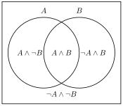
We can see both in the truth-table and the Venn diagram that if we calculate $\Prb(A \lor B)$ by adding up $\Prb(A)$ and $\Prb(B)$ we would be double-counting $\Prb(A \land B)$ . Rather, what we want to do is to add the first row of the truth-table (equivalently, the intersection of $A$ and $B$ ) just once, so that we end up with the probability of the region of the space of possibilities where either $A$ or $B$ are true:

Figure 5.1 The shaded region is $A \lor B$ .

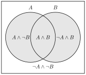
So, if we know $\Prb(\varphi)$ and $\Prb(\psi)$ , but we don’t know whether $\varphi$ and $\psi$ are mutually exclusive or not, how do we determine $\Prb(\varphi \lor \psi)$ ? Well, if just adding $\Prb(\varphi)$ and $\Prb(\psi)$ counts $\Prb(\varphi \land \psi)$ twice, we can just subtract it once, and so we have the following generalization of Additivity: $\Prb(\varphi \lor \psi) = \Prb(\varphi) + \Prb(\psi) - \Prb(\varphi \land \psi)$ , which for obvious reasons is sometimes called the inclusion-exclusion theorem:

Theorem 5.10. [Inclusion-exclusion theorem] For any two propositions $\varphi$ and $\psi$ , $\Prb(\varphi \lor \psi) = \Prb(\varphi) + \Prb(\psi) - \Prb(\varphi \land \psi)$ .

Proof. Left as an exercise for the reader. ◻

5.4 Conditional probability theorems

The inclusion-exclusion theorem determines $\Prb(\varphi \lor \psi)$ on the basis of three other quantities: $\Prb(\varphi), \Prb(\psi)$ , and $\Prb(\varphi \land \psi)$ . But, assuming we are given $\Prb(\varphi)$ and $\Prb(\psi)$ , how do we determine $\Prb(\varphi \land \psi)$ ? The next two theorems answer that question:

Theorem 5.11. For any two events $\varphi$ and $\psi$ :

if $\Prb(\psi) \neq 0$ , then $\Prb(\varphi \land \psi) = \Prb(\varphi \given \psi) \times \Prb(\psi)$ ;
if $\Prb(\psi) = 0$ , then $\Prb(\varphi \land \psi) = 0$ .

Proof. There are two possibilities— $\Prb(\psi) \neq 0$ or $\Prb(\psi) = 0$ —that we will consider in turn.

If $\Prb(\psi) \neq 0$ , then $\Prb(\varphi \land \psi) = \Prb(\varphi \given \psi) \times \Prb(\psi)$ .

Proof. Suppose that $\Prb(\psi) \neq 0$ . By Definition 4.2, since $\Prb(\psi) \neq 0$ , $\Prb(\varphi \given \psi) = \frac{\Prb(\varphi \land \psi)}{\Prb(\psi)}$ , which rearranges to $\Prb(\varphi \land \psi) = \Prb(\varphi \given \psi) \times \Prb(\psi)$ . ◻
If $\Prb(\psi) = 0$ , then $\Prb(\varphi \land \psi) = 0$ .

Proof. Suppose that $\Prb(\psi) = 0$ . As a matter of logic, $\psi$ is equivalent to $(\varphi \land \psi) \lor (\lnot \varphi \land \psi)$ . By Theorem 5.6, since $\psi$ is equivalent to $(\varphi \land \psi) \lor (\lnot \varphi \land \psi)$ , $\Prb(\psi) = \Prb((\varphi \land \psi) \lor (\lnot \varphi \land \psi))$ . $(\varphi \land \psi)$ and $(\lnot \varphi \land \psi)$ are mutually exclusive, and so by Additivity, since $(\varphi \land \psi)$ and $(\lnot \varphi \land \psi)$ are mutually exclusive, $\Prb((\varphi \land \psi) \lor (\lnot \varphi \land \psi)) = \Prb(\varphi \land \psi) + \Prb(\lnot \varphi \land \psi)$ . Thus, since $\Prb(\psi) = 0$ and $\Prb(\psi) = \Prb((\varphi \land \psi) \lor (\lnot \varphi \land \psi))$ , $\Prb(\varphi \land \psi) + \Prb(\lnot \varphi \land \psi) = 0$ . By Non-negativity, neither $\Prb(\varphi \land \psi)$ nor $\Prb(\lnot \varphi \land \psi)$ can be negative. Thus, since $\Prb(\varphi \land \psi) + \Prb(\lnot \varphi \land \psi) = 0$ , it must be that $\Prb(\varphi \land \psi) = \Prb(\lnot \varphi \land \psi) = 0$ . ◻

Since one of $\Prb(\psi) \neq 0$ or $\Prb(\psi) = 0$ must be true, (a) and (b) together establish the theorem. (When $\Prb(\psi) = 0$ the conditional probability $\Prb(\varphi \given \psi)$ is undefined, which is why the first claim of the theorem is restricted to the case $\Prb(\psi) \neq 0$ .) ◻

As a special case of Theorem 5.11, we can prove that when $\varphi$ is independent of $\psi, \Prb(\varphi \land \psi) = \Prb(\varphi) \times \Prb(\psi)$ :

Theorem 5.12. If an event $\varphi$ is independent of an event $\psi$ , then $\Prb(\varphi \land \psi) = \Prb(\varphi) \times \Prb(\psi)$ .

Proof. Let $\varphi$ be independent of $\psi$ . By Definition 5.2, since $\varphi$ is independent of $\psi$ , $\Prb(\varphi) = \Prb(\varphi \given \psi)$ . By Definition 5.2, $\Prb(\psi) \neq 0$ , and so by Theorem 5.11(a), $\Prb(\varphi \land \psi) = \Prb(\varphi \given \psi) \times \Prb(\psi)$ . By substituting $\Prb(\varphi)$ in for $\Prb(\varphi \given \psi)$ , we get $\Prb(\varphi \land \psi) = \Prb(\varphi) \times \Prb(\psi)$ . ◻

Going back to our discussion of the Gambler’s fallacy, Theorem 5.12 tells us that the probability of getting six tails in a row is exactly the same as the probability of getting five tails followed by heads, namely $0.5^{6} = \frac{1}{64}$ . To see why, let $T_{i}$ be the proposition that the $i$ th flip comes up tails. When we say that the flips of a fair coin are independent of each other, we mean that each flip is independent not just of each earlier flip taken separately, but of any combination of the earlier flips. So the sixth flip is independent of $T_{1} \land \ldots \land T_{5}$ , and by Theorem 5.12, $\Prb(T_{1} \land \ldots \land T_{6}) = \Prb(T_{1} \land \ldots \land T_{5}) \times \Prb(T_{6})$ . Applying the same reasoning to the earlier flips, $\Prb(T_{1} \land \ldots \land T_{6}) = 0.5^{6}$ . The same goes for five tails followed by heads. This is just what the Gambler’s fallacy overlooks: the conditional probability of heads on the sixth flip, given that the previous five were tails, is the same as the conditional probability of tails on the sixth flip, namely 0.5, because every flip is independent of the previous ones.

Ignoring cases where one of the propositions has probability 0 (which can give rise to strange independence relations), probabilistic independence is symmetric:

Theorem 5.13. For any two events $\varphi$ and $\psi$ , if $\Prb(\varphi) \neq 0$ and $\Prb(\psi) \neq 0$ , then $\varphi$ is independent of $\psi$ if and only if $\psi$ is independent of $\varphi$ .

Proof. Let $\Prb(\varphi) \neq 0$ and $\Prb(\psi) \neq 0$ . We prove the biconditional—that $\varphi$ is independent of $\psi$ if and only if $\psi$ is independent of $\varphi$ —by proving the two conditionals that constitute it.

$\varphi$ is independent of $\psi$ only if $\psi$ is independent of $\varphi$ .

Proof. Suppose that $\varphi$ is independent of $\psi$ . By Theorem 5.12, since $\varphi$ is independent of $\psi$ , $\Prb(\varphi \land \psi) = \Prb(\varphi) \times \Prb(\psi)$ . Since $\Prb(\varphi) \neq 0$ and $\Prb(\varphi \land \psi) = \Prb(\varphi) \times \Prb(\psi)$ , $\Prb(\psi) = \frac{\Prb(\varphi \land \psi)}{\Prb(\varphi)}$ . By Definition 4.2, since $\Prb(\varphi) \neq 0$ , $\Prb(\psi \given \varphi) = \frac{\Prb(\psi \land \varphi)}{\Prb(\varphi)}$ . By Theorem 5.6 and the logical equivalence of $\psi \land \varphi$ and $\varphi \land \psi$ , $\Prb(\psi \land \varphi) = \Prb(\varphi \land \psi)$ . Since $\Prb(\psi \land \varphi) = \Prb(\varphi \land \psi)$ and $\Prb(\psi \given \varphi) = \frac{\Prb(\psi \land \varphi)}{\Prb(\varphi)}$ , $\Prb(\psi \given \varphi) = \frac{\Prb(\varphi \land \psi)}{\Prb(\varphi)}$ . Since $\Prb(\psi) = \frac{\Prb(\varphi \land \psi)}{\Prb(\varphi)}$ and $\Prb(\psi \given \varphi) = \frac{\Prb(\varphi \land \psi)}{\Prb(\varphi)}$ , $\Prb(\psi) = \Prb(\psi \given \varphi)$ . By Definition 5.2, since $\Prb(\varphi) \neq 0$ and $\Prb(\psi) = \Prb(\psi \given \varphi)$ , $\psi$ is independent of $\varphi$ . ◻
$\varphi$ is independent of $\psi$ if $\psi$ is independent of $\varphi$ .

Proof. Exactly as the proof of (a) above, but with every instance of $\varphi$ replaced with $\psi$ , and every instance of $\psi$ replaced with $\varphi$ . ◻

By (a) and (b), we have it that $\varphi$ is independent of $\psi$ if and only if $\psi$ is independent of $\varphi$ . ◻

We say that $\varphi$ and $\psi$ are independent of each other (or just independent) when each of them is independent of the other. By Theorem 5.13, for propositions with non-zero probability this is the same as either one of them being independent of the other.

If a proposition $\varphi$ has probability 0, then it is independent of any proposition $\psi$ that has non-zero probability—see exercises below. But if $\Prb(\varphi) = 0$ , then the probability of any proposition conditional on $\varphi$ is undefined—see Definition 4.2—and so, by the definition of independence, no proposition at all is independent of $\varphi$ .

5.5 Solving problems

Armed with the axioms and theorems of the probability calculus, we can now solve a number of probabilistic problems. Let’s try a sample one:

Assume: $\Prb(H) = \frac{1}{2}, \Prb(G) = \frac{1}{5}, \Prb(\neg F) = \frac{3}{5}, \Prb(H \lor G) = \frac{3}{5}, \Prb(H \given F) = \frac{1}{2},$ and $F$ and $G$ are independent of each other.

What is $\Prb(H \land G)?$

Try it in the Probability Lab Follow the solution step by step in the lab.

The basic strategy for solving any problem like this is to:

Check what your goal is and note what’s involved in it.
Check what you already have and write down anything that involves the same elements as your goal.
Write down any axioms, theorems, and definitions that pertain to the kinds of things you are looking for or already have.
Check if you have everything written down that you need in order to solve for your goal.
If you do, just solve for your goal and you’re done!
If you don’t...
Repeat from step 1 with what you’re missing as your new goal.

Let’s apply this procedure to our sample problem. Our goal is to find out $\Prb(H \land G)$ , which involves $H, G$ , and conjunction. The second step is to check what we already have, which in this case is a lot. What is particularly relevant to our goal are the following:

$\Prb(H) = \frac{1}{2}$
$\Prb(G) = \frac{1}{5}$
$\Prb(H \lor G) = \frac{3}{5}$
$\Prb(H \given F) = \frac{1}{2}$
$F$ and $G$ are independent.

The third step is to examine the axioms, theorems and definitions to find if anything there is relevant to our goal.¹ Definition 4.2 concerns conjunction:

Conditional Probability: For any two propositions $\varphi$ and $\psi$ , provided that $\Prb(\psi) \neq 0$ ,

$\Prb(\varphi \given \psi) = \frac{\Prb(\varphi \land \psi)}{\Prb(\psi)}$

$\varphi$ and $\psi$ are metavariables ranging over propositions of PL. What we are interested in is the conjunction of $H$ and $G$ , so we should apply Definition 4.2 to those propositions:

Provided that $\Prb(G) \neq 0,$

$\Prb(H \given G) = \frac{\Prb(H \land G)}{\Prb(G)}$

We are also given that $\Prb(G) = \frac{1}{5}$ , so that the proviso of Definition 4.2 is satisfied. In order to solve for our goal— $\Prb(H \land G)$ —we need to know the values of $\Prb(H \given G)$ and $\Prb(G)$ . We know that $\Prb(G) = \frac{1}{5}$ , but we don’t know $\Prb(H \given G)$ . Maybe we’ll have to find $\Prb(H \given G)$ as an intermediate step in solving this problem, so let’s not completely abandon this line of reasoning, but we can set it aside for now to see if there is some easier way to do it.

Going back to our list of axioms and theorems that are relevant to our goal we find Theorem 5.10, according to which $\Prb(\varphi \lor \psi) = \Prb(\varphi) + \Prb(\psi) - \Prb(\varphi \land \psi)$ . Instantiating this theorem to $G$ and $H$ gives us:

$\Prb(H \lor G) = \Prb(H) + \Prb(G) - \Prb(H \land G)$

Does this help? It does, because we know that $\Prb(H \lor G) = \frac{3}{5}, \Prb(H) = \frac{1}{2}$ , and $\Prb(G) = \frac{1}{5}$ . Substituting in those values in the above formula gives us:

$\frac{3}{5} = \frac{1}{2} + \frac{1}{5} - \Prb(H \land G)$

Adding $\Prb(H \land G)$ and subtracting $\frac{3}{5}$ from both sides gives us our solution:

$\Prb(H \land G) = \frac{1}{2} + \frac{1}{5} - \frac{3}{5} = \frac{1}{2} - \frac{2}{5} = \frac{5}{10}- \frac{4}{10} = \frac{1}{10}$

Exercises

Suppose you are going to draw a card at random from a standard deck. For each pair of propositions, say whether they are independent or not.
1. $A$ = the card is red.
  $B$ = the card is an ace.
2. $A$ = the card is red.
  $B$ = the card is a diamond.
3. $A$ = the card is an ace.
  $B$ = the card is a spade.
4. $A$ = the card is a Queen.
  $B$ = the card is a face card.
Show solution
(a) independent; (b) not independent; (c) independent; (d) not independent.
For each of the following examples, say whether it’s an instance of the Gambler’s fallacy
1. You’re playing cards with your friends using a standard, randomly shuffled deck of 52 cards. You’re about half-way through the deck and no aces have been drawn yet. You conclude that an ace is due soon, and thus the probability the next card is an ace has gone up.
2. You’re holding a six-sided die, which you know to be fair. You’re going to roll it 60 times. You figure about 10 of those rolls should be threes. But after 59 rolls, you’ve rolled a three only five times. You figure that the probability of a three on the last roll has gone up: it’s higher than just $\frac{1}{6}$ .
3. You know the lottery numbers in New Jersey are selected using a fair process. So it’s really unlikely that someone will win two weeks in a row. Your friend won last week, so you conclude their chances of winning this week too are even lower than usual.
4. You’re visiting a new country where corruption is common, so you aren’t sure whether the lottery there is fair. You see on the news that the King’s cousin won the lottery two weeks in a row. You conclude that their chances of winning next week are higher than normal, because the lottery is rigged in their favor.
Show solution
(a) Not the fallacy: drawing without replacement, the probability that the next card is an ace is $4/26$ , not $4/52$ , so the earlier draws really are relevant. (b) The fallacy. (c) The fallacy (in its reverse form). (d) Not the fallacy.
Prove Theorem 5.10.

Show solution
$\varphi\lor\psi\equiv(\varphi\land\lnot\psi)\lor\psi$ , and the disjuncts are mutually exclusive, so $\Prb(\varphi\lor\psi)=\Prb(\varphi\land\lnot\psi)+\Prb(\psi)$ . Also $\varphi\equiv(\varphi\land\psi)\lor(\varphi\land\lnot\psi)$ , again mutually exclusive, so $\Prb(\varphi\land\lnot\psi)=\Prb(\varphi)-\Prb(\varphi\land\psi)$ . Substituting, $\Prb(\varphi\lor\psi)=\Prb(\varphi)+\Prb(\psi)-\Prb(\varphi\land\psi).$
Prove that if $\varphi$ has probability 0, then it is independent of any proposition $\psi$ with $\Prb(\psi) \neq 0$ . (Hint: by Theorem 5.8, $\Prb(\varphi \land \psi) \leq \Prb(\varphi)$ .)

Show solution
By monotonicity, $\Prb(\varphi\land\psi)\le\Prb(\varphi)=0$ , so $\Prb(\varphi\land\psi)=0$ . Hence $\Prb(\varphi\given\psi)=0=\Prb(\varphi)$ whenever $\Prb(\psi)>0$ .
Say whether the following event pairs are independent with each other. (All when rolling a pair of dice…)
1. “The sum of the faces is 5.” and “The first die comes up greater than 3, and the second less than 4.”
2. “The sum of the faces is 5.” and “The second die comes up less than 4.”
3. “The sum of the faces is 7.” and “The second die comes up odd.”
4. “The sum of the faces is 4.” and “The sum of the faces is 10.”
5. “The sum of the faces is 7 and the first die comes up odd.” and “The first die comes up greater than 2.”
Show solution
(a) independent ( $1/36=\frac16\cdot\frac16$ ); (b) not independent ( $1/12$ vs. $1/18$ ); (c) independent ( $1/12$ ); (d) not independent ( $0$ vs. $1/144$ ); (e) independent ( $1/18$ ).
Use the suppositional information to find the unknown probability.
1. Suppose that $J$ and $K$ are independent and $\Prb(K \given J) = 3/4$ . What is $\Prb(K)$ ? Practice in the Probability Lab
2. Suppose that $F$ and $G$ are independent and $\Prb(F) = 5/9$ . What is $\Prb(F \given G)$ ? Practice in the Probability Lab
3. What is $\Prb(H \lor \neg H)$ ? Practice in the Probability Lab
4. Suppose that $F$ and $G$ are mutually exclusive, $\Prb(F) = 1/4$ , and $\Prb(G) = 2/3$ . What is $\Prb(F \lor G)$ ? Practice in the Probability Lab
5. Suppose that $J$ and $K$ are mutually exclusive, $\Prb(J \lor K) = 3/8$ , and $\Prb(J) = 1/4$ . What is $\Prb(K)$ ? Practice in the Probability Lab
6. Suppose that $\Prb(X) = 2/3$ and $\Prb(X \land Y) = 3/7$ . What is $\Prb(Y \given X)$ ? Practice in the Probability Lab
7. Suppose that $\Prb(F \land G) = 2/5$ and $\Prb(G \given F) = 3/4$ . What is $\Prb(F)$ ? Practice in the Probability Lab
8. What is $\Prb(H \land \neg H)$ ? Practice in the Probability Lab
9. Suppose that $F$ and $G$ are mutually exclusive. What is $\Prb(G \land F)$ ? Practice in the Probability Lab
10. Suppose that $\Prb(J) = 4/7$ . What is $\Prb(\neg J)$ ? Practice in the Probability Lab
11. Suppose that $\Prb(R) = 1/3$ and $R$ and $S$ are logically equivalent. What is $\Prb(S)$ ? Practice in the Probability Lab
12. Suppose that $\Prb(G) = 1/3$ and $F$ and $G$ are logically equivalent. What is $\Prb(\neg F)$ ? Practice in the Probability Lab
13. Suppose that $\Prb(J) = 5/8$ , $\Prb(K) = 3/4$ , and $\Prb(J \land K) = 3/8$ . What is $\Prb(J \lor K)$ ? Practice in the Probability Lab
14. Suppose that $\Prb(M) = 2/3$ , $\Prb(L \land M) = 1/2$ , and $L$ is independent of $M$ . What is $\Prb(L)$ ? Practice in the Probability Lab
15. Suppose that $\Prb(S \given R) = 1/3$ and $\Prb(S) = 1/3$ . Is $R$ independent of $S$ ? Practice in the Probability Lab
16. Suppose that $\Prb(G \land H) = 1/3$ , $\Prb(G) = 1/2$ , and $\Prb(H) = 1/3$ . Is $H$ independent of $G$ ? Practice in the Probability Lab
17. Suppose that $\Prb(J \given K) = 1/2$ , $\Prb(J) = 1/3$ , and $\Prb(K) = 3/5$ . What is $\Prb(K \given J)$ ? Practice in the Probability Lab
18. Suppose that $\Prb(L \given M) = 5/9$ , $\Prb(M \given L) = 2/3$ , and $\Prb(M) = 3/5$ . What is $\Prb(L)$ ? Practice in the Probability Lab
Show solution
(a) $3/4$ ; (b) $5/9$ ; (c) $1$ ; (d) $11/12$ ; (e) $1/8$ ; (f) $9/14$ ; (g) $8/15$ ; (h) $0$ ; (i) $0$ ; (j) $3/7$ ; (k) $1/3$ ; (l) $2/3$ ; (m) $1$ ; (n) $3/4$ ; (o) yes; (p) no (e.g. $\Prb(H\given G)=2/3\neq1/3=\Prb(H)$ ); (q) $9/10$ ; (r) $1/2$ .
Let the following be true: $\Prb(H) = 1/2$ , $\Prb(G) = 1/5$ , $\Prb(\neg F) = 3/5$ , $\Prb(H \lor G) = 3/5$ , $\Prb(H \given F) = 1/2$ , $F$ is independent of $G$ . Find the values of the probabilities below.
1. $\Prb(F)$ Practice in the Probability Lab
2. $\Prb(F \land G)$ Practice in the Probability Lab
3. $\Prb(F \land H)$ Practice in the Probability Lab
4. $\Prb(G \given F)$ Practice in the Probability Lab
5. $\Prb(F \given H)$ Practice in the Probability Lab
Show solution
(a) $2/5$ ; (b) $2/25$ ; (c) $1/5$ ; (d) $1/5$ ; (e) $2/5$ .
Let the following be true: $\Prb(J) = 3/5$ , $\Prb(K) = 2/5$ , $\Prb(L \land K) = 3/10$ , $\Prb(L \lor K) = 3/5$ , $\Prb(L \given J) = 2/3$ , $K$ is logically equivalent to $\neg M$ , and $J$ is independent of $M$ . Find the values of the probabilities below.
1. $\Prb(M)$ Practice in the Probability Lab
2. $\Prb(J \given M)$ Practice in the Probability Lab
3. $\Prb(J \given L)$ Practice in the Probability Lab
4. $\Prb(K \lor M)$ Practice in the Probability Lab
5. $\Prb(J \land L)$ Practice in the Probability Lab
Show solution
(a) $3/5$ (this is $\Prb(M)$ ); (b) $3/5$ ( $\Prb(J\given M)$ ); (c) $4/5$ ( $\Prb(J\given L)$ ); (d) $1$ ( $\Prb(K\lor M)$ ); (e) $2/5$ ( $\Prb(J\land L)$ ). Along the way, $\Prb(L)=1/2$ .
Let the following be true: $\Prb(X) = 1/2$ , $\Prb(Y) = 1/2$ , $\Prb(X \land Y) = 1/4$ .
1. Are $X$ and $Y$ mutually exclusive? Practice in the Probability Lab
2. What is $\Prb(X \lor Y)$ ? Practice in the Probability Lab
Show solution
(a) No. (b) $3/4$ .